

4Fundamental limitations of small antennas
4.1Fundamental limitations
It is commonly understood that as antennas reduce in size, antenna gain and efficiency will degrade and the bandwidth tends to be narrower. Then, a question arises how small a dimension an antenna can take for practical use? Or, what will happen when the antenna dimension is limitlessly reduced? One answer was given by J. D. Kraus, who showed that a small antenna could have effective aperture of as high as 98 percent of that of a half-wave dipole antenna, if the antenna could be perfectly matched to the load [1]. It suggests that however small an antenna is, the antenna can intercept almost the same power (only 8 percent less) as a half-wavelength dipole does. In other words, there seems to be no limitation in reducing the antenna size so long as the antenna could be perfectly matched. Unfortunately, the perfect matching is impossible when an antenna becomes extremely small, because the smaller the antenna size tends to be, the harder the antenna matching will become, as was mentioned before. In addition, losses existing in the antenna structure and the matching circuit will exceed the radiation resistance, resulting in significant reduction of the effective aperture that corresponds to reduction of the radiation power and the degradation of the radiation efficiency. Regarding the antenna impedance, increase in reactive component and decrease in the resistive component results in high Q, and as a consequence bandwidth will be narrowed. Thus, the size reduction of an antenna also affects Q and the bandwidth as well. Then it is rather natural to say that there is a fundamental limitation applying to the size reduction of antenna dimensions. This implies in turn that antenna gain, efficiency, Q, and the bandwidth are bounded by the antenna dimensions. Parameters that concern fundamental limitations of small antennas are antenna Q, relative bandwidth (RBW), radiation efficiency η, and the antenna size ka, where a is the radius of a sphere circumscribing the antenna. In summary, relationships between these parameters and the antenna size are roughly approximated, when ka is much smaller than unity, as follows:
(a)Q is proportional to (ka)−3
(b)RBW is proportional to (ka)3, since RBW nearly equals 1/Q
(c)η is proportional to (ka)4
24 |
Fundamental limitations of small antennas |
|
|
a
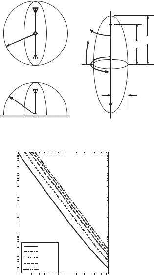
Figure 4.1 A sphere model enclosing an antenna of radius a.
C L
A=πa2
2a
b
V=Ab
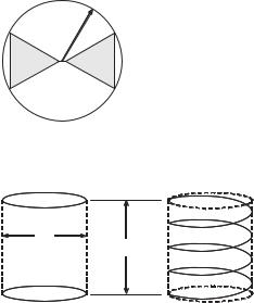
Figure 4.2 A capacitor and an inductor with a cylindrical shape [2].
4.2Brief review of some typical work on small antennas
Systematic analysis of small antennas was probably first made by H. A. Wheeler, who extensively treated small antennas practically as well as theoretically [2–5]. One of his notable works is on the limitation of small antennas. He showed that the size reduction of an antenna directly limits the radiation power factor (RPF), a ratio of the radiated power to the reactive power, implying that the radiation efficiency is constrained by the antenna size. It was also shown that the RPF equals the reciprocal of Q, thus the size reduction of antenna limiting Q corresponds to a limitation of the RBW depending on the antenna size.
By assuming a sphere model of radius a, which encloses a small antenna as shown in Figure 4.1, Wheeler derived Q for the most limiting case as
Q = 1/(ka)3. |
(4.1) |
This equation indicates that Q is inversely (cubic) proportional to the size of an antenna, so the antenna size imposes the fundamental limitation of the bandwidth.
Wheeler didn’t work only on the theory of small antennas, but also on design and development of practical antennas. From the early to mid twentieth century, almost all antennas were “small antennas” because of their lower operating frequencies and electrically small size. Wheeler’s development was large-sized antennas; however they were electrically small. His antennas were designed based on the concept introduced by himself.
Wheeler considered small antennas to behave as a capacitor C or an inductor L, which was assumed to be circumscribed by a cylinder-shaped volume, as shown in Figure 4.2

4.2 Brief review of some typical work on small antennas |
25 |
|
|
a V
 μ = ∞
μ = ∞
(a) |
(b) |
Figure 4.3 A spherical coil (a) without and (b) with a magnetic core filled [2, 5].
0.04λ
 C
C
pm = 0.001
Figure 4.4 A loop coil ferrite-loaded antenna [5].
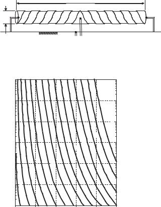
[2]. He derived the radiation power factor (RPF), which is a ratio of the radiated power to the reactive power, for the C or the L types of small antennas [2, 5] and showed that it is directly proportional to the volume. His idea of the cylindrical radiator is extended to create a self-resonant helical coil that would radiate equal power in both TE and TM modes in phase quadrature so that circular polarization is yielded [6]. This type of antenna was later named as the Normal Mode Helical Antenna (NMHA) by J. D. Kraus [7]. Wheeler designed the NMHA for the first US communications satellite Telstar, on which the antenna handled the command and telemetry systems in the VHF band. He also invented a spherical coil, in which a magnetic core was filled (Figure 4.3) [5, 8]. Another practical antenna he developed was a one-turn loop of wide strip (Figure 4.4) [9], which was used for the oscillator of the proximity fuse in the nose cone on a small rocket [10]. A long coil on a ferrite core was commonly used for the radio-broadcasting receiver in the frequency range of 0.55–1.5 MHz and VLF. Some types of long coil ferrite-loaded antennas were found to be useful for horizontal mount on vehicles (Figure 4.5) [11]. Also, a VLF loop was applied to submarines [12].
Chu followed Wheeler’s work on small antennas. He also analyzed the limitations of small antennas, but more exactly than Wheeler. In his analysis [13], he assumed a vertically polarized dipole antenna circumscribed by a sphere of radius a, and expressed the radiation field produced outside the sphere with a spherical function expansion, which can describe the fields with a sum of the spherical modes. By introducing the
26 |
Fundamental limitations of small antennas |
|
|
4 turns |
b = 0.36 m |
3 turns |
|
0.04 m
Figure 4.5 Over turn loop of a wide strip [5].
|
106 |
|
|
|
|
|
|
|
|
105 |
|
|
|
|
|
|
|
|
10 |
4 |
|
|
|
|
|
9 |
|
|
|
|
|
|
|
||
|
|
|
|
|
|
|
2 |
|
|
|
|
|
|
|
|
|
= |
|
|
|
|
|
|
|
|
n |
|
|
|
|
|
|
|
|
7 |
|
|
|
|
|
|
|
|
2 |
|
|
|
|
|
|
|
5 |
|
|
|
|
|
|
|
3 |
2 |
|
|
|
|
|
|
|
|
|
|
n |
10 |
3 |
|
|
|
2 |
|
|
|
|
|
1 |
|
|
|||
Q |
|
|
|
|
|
|
||
|
|
|
9 |
2 |
|
|
||
|
|
|
|
|
|
|
|
|
|
|
|
|
|
1 |
|
|
|
|
|
|
|
|
7 |
|
|
|
|
|
|
|
|
1 |
|
|
|
|
|
|
|
|
5 |
|
|
|
|
|
|
|
|
1 |
|
|
|
|
|
|
|
3 |
|
|
|
|
|
10 |
2 |
|
1 |
|
|
|
|
|
|
1 |
|
|
|
|
||
|
|
|
1 |
|
|
|
|
|
|
|
|
9 |
|
|
|
|
|
|
|
|
|
|
|
|
|
|
|
|
|
|
7 |
|
|
|
|
|
|
|
5 |
|
|
|
|
|
|
10 |
1 |
3 |
|
|
|
|
|
|
1 |
|
|
|
|
|
||
|
|
|
|
|
|
|
||
|
|
|
|
|
|
|
|
|
|
100 |
5 |
10 |
15 |
|
20 |
25 |
|
|
|
0 |
|
|||||
|
|
|
|
|
2πa/λ |
|
|
|
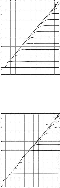
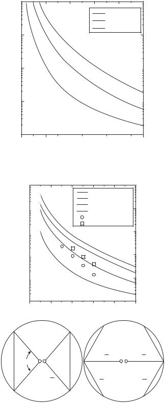
Figure 4.6 Lowest obtainable Q with antenna dimension maximum [13].
equivalent circuits for each mode, the modal impedance and the antenna Q for each mode are derived. He obtained the lowest possible Q, highest obtainable Gain G and the highest obtainable G/Q, and gave graphs as shown in Figures 4.6–4.8.
Chu’s results have been understood as the important derivation that provides the lowest obtainable Q that concerns the highest obtainable bandwidth, and the highest achievable G/Q, with maximum dimensions of antenna, although his analysis is accurate only for the lowest mode, whereas it includes rough approximations for the higher modes.
King worked extensively on linear antennas both theoretically and numerically [14– 15], including small antennas. He showed fundamentals of linear antennas, demonstrating current distributions on antenna elements, numerical values of impedance, and Q for various types and dimensions of linear antennas with theoretical and numerical data, and figures of these. He defined “Electrically Short Antenna,” instead of “Electrically Small Antenna,” as one that has the maximum length ka smaller than 0.5. The impedance of a small dipole antenna was given previously in Figure 3.2. Table 4.1 shows resistance
4.2 Brief review of some typical work on small antennas |
27 |
|
|
GAIN
16 |
N = 27 |
|
N = 25 |
14 |
N = 23 |
N = 21 |
|
|
N = 19 |
12 |
N = 17 |
|
|
|
N = 15 |
10 |
N = 13 |
|
|
8 |
N = 11 |
|
|
|
N = 9 |
6 |
N = 7 |
|
|
4 |
N = 5 |
|
|
|
N = 3 |
2 |
N = 1 |
|
0 


 0 2 4 6 8 10 12 14 16 18 20 22 24
2πa/λ
Figure 4.7 Highest obtainable gain with antenna dimension maximum [13].
G/Q
16 |
N = 27 |
||
|
|||
|
N = 25 |
|
|
14 |
N = 23 |
|
|
N = 21 |
|
19 |
|
|
= |
||
|
N |
||
|
|
||
|
|
|
|
12 |
N = 17 |
||
|
N = 15 |
|
|
10 |
N = 13 |
|
|
|
|
|
|
8 |
N = 11 |
|
|
|
|
|
|
|
N = 9 |
|
|
6 |
N = 7 |
|
|
|
|
|
|
4 |
N = 5 |
|
|
|
|
|
|
|
N = 3 |
|
|
2 |
N = 1 |
|
|
0 


 0 2 4 6 8 10 12 14 16 18 20 22 24
2πa/λ
Figure 4.8 Highest obtainable G/Q with antenna dimension maximum [13].

28 |
Fundamental limitations of small antennas |
|
|
Table 4.1 Resistance and reactance for electrically short antennas [14, 15]
|
|
(ohm.) |
a |
Xa |
Ra |
|
|
|
0 |
–∞ |
0 |
0.1 |
–3945 |
0.183 |
0.2 |
–1950 |
0.732 |
0.3 |
–1274 |
1.66 |
0.4 |
–929 |
2.97 |
0.5 |
–716 |
4.67 |
0.6 |
–569 |
6.80 |
0.7 |
–460 |
9.35 |
0.8 |
–373.7 |
12.38 |
0.9 |
–303.5 |
15.82 |
1.0 |
–238.2 |
19.90 |
|
|
|
Ra and reactance Xa for electrically short antennas of length 2h and radius a calculated by
Ra = 18.3β02h2 |
1 |
+ 0.086β02h2 |
|
(4.2) |
|||
|
a = − |
60 |
( |
3.39) |
|
|
|
|
|
β0h |
|
|
|||
and X |
|
|
|
|
|
|
(4.3) |
where = 2 ln (2h/a) and
β0 = 2π/λ0.
King gave the expression for antenna Qr at the resonance in terms of the impedance [16] by analogy with a lumped-constant RLC circuit as
Qr = |
|
2R dω res . |
(4.4) |
|
|
ω d X |
|
Here X = ωL − 1/ωC and ωL = 1/ωC at resonance.
Collin and Rothschild improved previously given theory for obtaining Q based on the field rather than the equivalent circuit [17]. They calculated Q for cases where both TE and TM modes are used for excitation, and derived it for the lowest mode as
Q = 1/(ka)3 + 1/(ka). |
(4.5) |
This Q represents the minimum possible value. Fante generalized their treatment to include both TE and TM modes, and found that equal excitation of TE and TM modes does not provide Q of half the value for the excitation of either mode alone. The actual result was somewhat larger than half the original value.
Hansen simplified Chu’s expression for calculating Q [18]. He stated that when ka is roughly less than unity and only the lowest TM mode propagates, Q is expressed by
Q = [1 + 3(ka)3]/(ka)3[1 + (ka)2]. |
(4.6) |
4.2 Brief review of some typical work on small antennas |
29 |
|
|
Q
100
60
40
 dipole
20
10 |
|
|
|
|
|
|
|
|
|
|
|
|
|
|
|
|
|
|
|
|
|
|
|
|
|
|
|
|
|
|
|
|
|
|
|
6 |
|
|
|
|
|
|
|
|
|
|
dipole |
|
|
|
|
|
|
4 |
|
|
|
|
|
|
|
|
|
|
|
|
|
|
|
|
|
|
|
|
|
|
|
|
|
|
|
|
Gaubau antenna |
||||||
2 |
|
|
5 |
10 |
50 |
|
η = 100% |
|
|
|
|||||||
|
|
|
|
|
|
|
|||||||||||
1 |
|
|
|
|
|
|
|
|
|
|
|
|
|
|
|
|
|
0.1 |
0.3 |
0.5 |
0.7 |
0.9 |
1.1 |
1.3 |
1.5 |
||||||||||
κa
Figure 4.9 Antenna Q of a short dipole antenna [18].
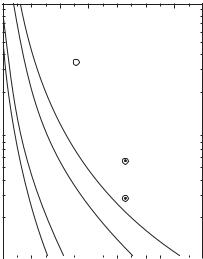
Hansen concluded that the value of Q would be halved when TM and TE modes are equally excited. He illustrated Q with respect to the antenna size ka along with the radiation efficiency η as the parameter (Figure 4.9). This figure is useful and convenient for finding antenna Q, thus bandwidth, and the efficiency in relation with antenna size when designing a small antenna of a given size.
McLean corrected some previous derivations obtained by Wheeler, Chu, and Hansen, as he thought their results were too rough to establish fundamental limits of Q because of the simple assumption or approximation [19]. He derived Q as
Q = [1 + 2(ka)3]/(ka)3[1 + (ka)2]. |
(4.7) |
He concluded that when ka is very small, there is not much difference between the previous derivations and his own derivation, and equation (4.7) is an exact expression of the lower bound on Q for a given antenna size.
Folts and McLean used a prolate spheroid that would better approximate an actual antenna like a dipole antenna (Figure 4.10) and evaluated Q vs. ka [20]. They considered that Q previously obtained was not really close to the verifiable values for many antennas, because the volume of a sphere surrounding an antenna was not fully utilized, and that made the value of Q larger than was expected. Figure 4.11 depicts Q, using the parameter a/b, where a and b respectively denote the major axis and the minor axis of the prolate spheroid.
Thiele obtained Q by a different method, as he thought that previously obtained Q was far from that of actual antennas, because the current distributions were not taken into consideration in the calculation [21]. He used the superdirective ratio SDR for
30 |
Fundamental limitations of small antennas |
|
|
|
|
ε |
a |
η |
a |
|
|
f |
(a) |
|
φ |
|
|
|
a |
|
b |
|
|
|
(b) |
|
(c) |
Figure 4.10 A prolate spheroidal model approximating a small monopole and dipole antenna [20].
|
106 |
|
|
|
105 |
|
|
Factor Q |
104 |
|
|
103 |
|
|
|
Quality |
102 |
|
|
|
|
ab = 1 |
|
|
101 |
ab = 3 |
|
|
|
ab = 10 |
|
|
|
ab = 30 |
|
|
100 |
ab = 100 |
|
|
0.1 |
1 |
|
|
0.01 |
Electrical height κa, radians
Figure 4.11 Q of a prolate spheroidal model with respect to electrical length ka [20].
calculating Q, based on the concept that the radiation energy is concerned with the visible region in the radiation field, while the total stored energy is concerned with the invisible region. The calculated Q for a thin dipole antenna in terms of X/R McLean’s result, lower bound for an ideal dipole with uniform current distribution, and far field Q for a dipole with sinusoidal current distribution are shown in Figure 4.12. Figure 4.13 depicts Q for a thin dipole of different radius, end-loaded dipole, and bow-tie antenna, respectively. In the figure, McLean’s Q was drawn as a comparison.
|
104 |
|
103 |
A |
102 |
Q |
|
|
101 |
100
0.00.2
Figure 4.12 Q vs. βa [21].
105
104 
103 
QA
102 
101 
100
0.0 0.2
(Bow-tie)
90°
a =
L
2
Dipole |X/R|
Far-field Q
McLean
|
|
Typical |
Wire |
|
|
|
|
|||
|
|
|
Q |
|||||||
|
|
|
|
|
|
|||||
|
|
|
|
Far |
Dipole |
|||||
|
|
|
|
|
- |
|
|
|
|
|
|
|
|
|
|
field |
|
|
|
||
|
|
|
|
McLean |
|
|
|
|||
|
|
|
|
|
|
|
|
|
||
|
|
|
|
|
|
|
|
|
|
|
0.4 |
0.6 |
|
0.8 |
1.0 |
||||||
|
βa or πL/λ |
|
|
|
|
|
|
|
||
Radius = .00005λ
Radius = .001λ
Far-field Q
McLean Equation
End-Loaded Dipole
Bowtie
|
|
|
Q |
|
|
Far |
|
|
|
|
- |
|
|
|
McLean |
Equation |
field |
|
|
|
|
|
||
|
|
|
|
|
0.4 |
0.6 |
0.8 |
1.0 |
|
βa |
|
|
|
|
|
|
(End-loaded |
|
|
|
|
dipole) |
|
|
|
L |
|
|
L |
|
2 |
|
|
2 |
|
L |
|
a = |
L |
|
2 |
|
2 |
|
Figure 4.13 Q vs. βa or π L/λ (a: radius, L: diameter of a sphere enclosing the radiator) [21].
32 |
Fundamental limitations of small antennas |
|
|
z
|
|
|
|
y |
|
|
|
|
driven |
|
|
|
|
|
z |
|
source |
|
|
|
|
|
|
2a |
|
|
|
|
driven |
|
|
|
y |
|
|
source |
|
|
|
|
|
|
|
|
|
|
driven |
|
|
2ao |
|
|
|
x |
source |
|
|
|
|
|
|
||
x |
|
|
|
|
|
|
|
|
|
|
a |
|
|
|
|
|
2ao |
|
|
|
|
x |
|
|
|
|
|
|
|
||
|
|
|
|
|
|
|
ground |
(a) |
|
|
|
(b) |
|
|
(c) |
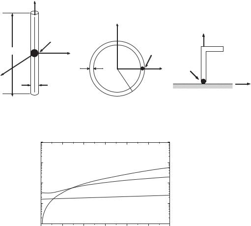
Figure 4.14 Antenna models used for evaluation of Q: (a) a dipole, (b) a loop, and (c) inverted-L |
|||||||
[23]. |
|
|
|
|
|
|
|
103 |
|
|
|
|
|
|
|
102 |
|
|
|
|
|
|
|
|
|
|
|
Gnorm |
|
|
|
101 |
|
|
|
max |
|
|
|
|
|
|
|
Gdir |
|
|
|
100 |
|
|
|
Gomnmax |
|
|
|
10−1 |
|
|
|
|
|
|
|
0 |
1 |
2 |
3 |
4 |
5 |
|
6 |
κa
Figure 4.15 Maximum obtainable gain [22].
Geyi studied Q [22–24] rigorously by introducing complex power balance relations into an antenna structure and derived an expression of Q for several typical antennas such as a dipole, small loop, and an inverted-L antenna as Figure 4.14 shows [23]. He also discussed physical limitations of small antennas, and derived minimum possible Q for both TE and TM modes excited by the antenna, and the ratio of maximized G/Q and normal gain, respectively, and his results are shown in Figures 4.15, 4.16 and 4.17 [22–24].
Best discussed Q of electrically small linear and elliptically polarized spherical dipole antennas, based on the concept that the Q of a resonant electrically small dipole antenna can be minimized by utilizing the occupied spherical volume to the greatest possible extent with the antenna geometry. He demonstrated a self-resonant (at 300 MHz)
4.2 Brief review of some typical work on small antennas |
33 |
|
|
103 |
|
|
|
|
|
|
|
|
|
|
|
|
|
|
|
|
|
|
|
|
|
|
|
102 |
|
|
|
|
|
|
|
max |
G |
|
|
|
|
|
|
|
|
|
|
|
|
||
|
|
|
|
|
|
|
|
|
|
|
|
|
|
|
|
|
|
|
|||||
|
|
|
|
|
|
|
|
Q |
dir |
|
|
|
|
|
|
|
|
|
|
|
|||
|
|
|
|
|
|
|
|
|
|
|
|
|
|
|
|
|
|
|
|
|
|
||
101 |
|
|
|
|
|
|
|
|
|
max |
G |
|
|
|
|
|
|
|
|
|
|
||
|
|
|
|
|
|
|
|
|
|
|
|
|
|
|
|
|
|
|
|||||
|
|
|
|
|
|
|
|
|
|
|
|
|
|
|
|
|
|
||||||
|
|
|
|
|
|
|
|
|
|
|
|
|
|
|
|
||||||||
100 |
|
|
|
|
|
|
|
|
|
Q |
|
omn |
|
|
|
|
|
||||||
|
|
|
|
|
|
|
|
|
|
|
|
|
|
|
|
|
|
||||||
|
|
|
|
|
|
|
|
|
|
|
|
|
|
|
|
|
|||||||
|
|
|
|
|
|
|
|
|
|
|
|
|
|
|
|
|
|
||||||
10−1 |
|
|
|
|
|
|
|
|
|
|
|
|
|
|
|
|
|
|
|
|
|
|
|
0 |
1 |
2 |
3 |
|
|
4 |
5 |
6 |
|||||||||||||||
|
|
|
|
|
|
|
|
κa |
|
|
|
|
|
|
|
|
|
|
|
||||
Figure 4.16 Maximum obtainable G/Q [22].
103 
102 
101 |
|
|
|
|
Qmindir |
|
|
|
Qomnmin |
|
|
|
|
|
||||
|
|
|
|
|
|
|
|
|
|
|
|
|||||||
|
|
|
|
|
|
|
|
|
|
|
|
|
||||||
100 |
|
|
|
|
minQ |
|
|
|
|
|
|
|
|
|||||
|
|
|
|
|
|
|
|
|
|
|
|
|||||||
10−1 |
|
|
|
|
|
|
|
|
|
|
|
|
|
|
|
|||
|
|
|
|
|
|
|
|
|
|
|
|
|
|
|
|
|
|
|
0 |
1 |
2 |
3 |
4 |
5 |
6 |
||||||||||||
|
|
|
|
|
|
|
|
κa |
|
|
|
|
|
|
|
|
||
Figure 4.17 Minimum possible Q [22].
four-arm folded linearly polarized spherical dipole antenna that exhibits an impedance 47.5 , an efficiency of 97.4%, and Q of 87.3, which is within 1.5 times the fundamental lower bound at a value ka of 0.263 [25]. This antenna may have the lowest Q that can be realized with a practical antenna. He also showed that a self-resonant (at 300 MHz) elliptically polarized antenna exhibits Q within two times the lower bound. The antenna has an efficiency of 95% and an impedance of 61.5 .
Best also treated Q and bandwidth in terms of antenna impedance and gave relationships between Q and VSWR fractional bandwidth (FBW) [26–27]. He discussed the upper bound of VSWR FBW for loss-free antennas and showed it to be
|
|
2√ |
|
(ka)3 |
(ka)3 |
|
s − 1 |
|
||||
FBW |
|
β |
(4.8) |
|||||||||
|
|
|
|
|
|
|
|
|
||||
V ub = |
1 + (ka)2 = |
1 + (ka)2 √s |
||||||||||
|
|
|||||||||||

34 |
Fundamental limitations of small antennas |
|
|
Figure 4.18 An antenna model used for evaluating minimum Q [29].
where s denotes VSWR. The maximum available FBW when a number of tuned circuits are applied to the matching circuit in order to increase the BW is given by
FBWV max |
|
1 |
|
|
π |
|
|
|
(ka)3 |
|
π |
|
|
π (ka)3 |
. |
(4.9) |
|
|
= Q ln |
s−+1 |
= |
1 + (ka) |
|
ln s−+1 |
≈ ln s−+1 |
|
|
|
|||||||
Best further has given evaluation of Q for various different dipole-type antennas [25, 28].
Thal commented that previous treatment of Q ignored the energy inside the sphere, resulting in considerably higher Q limit for realizable antennas than the minimum values predicted by the previous work. He then derived minimum Q values that include the contributions of energy within the sphere by using an antenna model formed by conducting thin wires on the surface of a sphere [29]. The antenna model he used is depicted in Figure 4.18. He used the equivalent circuits representing the antenna system valid for both outside and inside the sphere, accounting for the mode energy stored inside the sphere. He defined stricter limits that apply to a class of antennas consisting of conductors arranged to conform to a spherical surface and showed that the new limit he derived should be helpful for estimating the minimum Q of wire antenna configurations not necessarily exactly spherical but reasonably approximating the configuration of a sphere.
Thal, after his discussion on the limit of Q [29], explored the relationships between phase, gain, bandwidth, and the Q lower bound, particularly for electrically small antennas [30], and provided general theory and numerical examples giving a lower bound on the Q of any antenna with coupled TM–TE modes as a function of the electrical radius ka and the relative phases of the radiated mode fields, by which the gain is determined. He showed values of radiation Q with respect to ka from 0.05 to 0.65 and the minimum Qs for TM and TE mode, respectively, are 1.5 and 3 times Qchu, which is given by Chu [17].
Hansen and Collin also calculated internal stored energy and provided exact formulas for total stored energy Q for TM modes and an approximate formula for the Q of the lowest mode [31]. The calculation was based on the previous work [17], by which formulas for the Q values of TM and TE modes are derived for a case where these modes

4.2 Brief review of some typical work on small antennas |
35 |
|
|
1000
QNEW
100
Q
QCHU
10 |
|
|
|
|
|
0 |
–1 |
–2 |
–3 |
–4 |
–5 |
|
|
|
ka |
|
|
Figure 4.19 Q calculated by using Equation (4.10) and Qchu [31].
are excited by current sheets on a sphere and include the stored reactive energy within the sphere. Then by following Thal [29], new formulas to express Q for TM modes are derived [31], by treating the reactive power inside the sphere circumscribing the antenna, whereas Chu’s calculation did not include that. Thus the Q is given by the Qchu plus an additional term which corresponds to the internal reactive energy. This formula is simplified to an approximate formula similar to (4.5), which can be expressed by
|
3 |
|
√ |
|
|
|
|
Q = 3/2(ka) |
+ 1/ |
2(ka). |
(4.10) |
||||
|
|
||||||
The value of Q with respect to the antenna dimension ka is depicted in Figure 4.19 [31], where the Qchu is also given as a comparison.
Discussions on the Q of radiating structures have continued. Gustafsson gave new physical bounds for antennas of arbitrary shape and illustrated numerical examples [32]. He presented physical bounds for antennas circumscribed by the rectangular parallelepiped, finite cylinders, and planar rectangles. The theory can directly be applied to analyze the potential performance of different antenna geometries using pattern and polarization diversity.
Vandenbosch derived general and rigorous expressions for calculating the reactive energy stored in the electromagnetic field around an arbitrary source device [33]. A straightforward application is to investigate the energies and Q of radiating structures in

36Fundamental limitations of small antennas
terms of topology of the device. The expressions can be applied to much more general topology, particularly for small antennas.
Kim et al. studied Q of electrically small current distributions and practical antenna designs radiating the TE10-mode magnetic dipole field, and derived closed form expressions for the internal and external electric and magnetic stored energies and radiated power by a spherical, electric surface current density enclosing a magneto-dielectric core [34]. This result leads to determining the Q for arbitrary values of ka. He demonstrated that for a given size of antenna and permittivity, there is an optimum permeability that ensures the lowest possible Q, and this optimum permeability is inversely proportional to the square of the antenna electrical radius. With permittivity of unity, the optimum permeability yields the lowest bound of Q for a magnetic dipole antenna with a magneto-dielectric core. He obtained by simulation Q of 1.24 times Qchu for the TE10-mode multi-arm spherical helix antenna with a magnetic core, for ka of 0.192.
Yaghjian obtained general expressions for the lower bounds on Q of electrically small electric and magnetic-dipole antennas confined to an arbitrary shaped volume V which are excited by general sources or by global electric current sources alone [35]. He showed that the lower bound expressions depend only on the direction of the dipole moment with respect to V, electrical size of V, and per unit volume static PEC (Perfect Electric Conductor) and PMC (Perfect Magnetic Conductor) electric and magnetic polarizabilities of V. He provided new expressions of the lower bound Q for electrically small electric and magnetic dipole antennas, and sources restricted to global surface currents.
Stuart and Yaghjian investigated the effect of a thin shell of high permeability magnetic material on Q for the electrically small, top-loaded electrical dipole antenna [36]. The magnetic polarization currents induced in the thin shell of magnetic material reduce the internal stored energy, leading to a lower Q. It was shown that for the case of spherical antennas, Q approaches Qchu.
Kim and Breinbjerg found that the lower bound for radiation Q of spherical magnetic dipole antennas with pure solid magnetic core could approach Qchu as the antenna electrical size decreases [37]. With properly selected permeability, the antenna can exhibit a lower Q than the air-core magnetic and electric dipole antennas of the same size in the range of ka < 0.863.
So far, Chu’s limitation has been understood as the lowest achievable Q for an antenna of given size, which, however, would be impossible in reality to achieve. Design of small antennas is an exercise in finding new techniques to approach Chu’s limitations Qchu as closely as possible with small antennas. The main issues would be study on the antenna shape, current distributions on it, and relationships with radiation efficiency.
References
[1]J. D. Kraus, Antennas, 3rd edn., McGraw-Hill, 2002, pp. 30–33.
[2]H. A. Wheeler, Fundamental Limitations of Small Antennas, Proceedings of IRE, vol. 35, Dec 1947, pp. 1479–1484.

References 37
[3]H. A. Wheeler, Small Antennas, in H. Jasik (ed.), Antenna Engineering Handbook, 2nd edn., McGraw-Hill, 1984, chapter 6.
[4]H. A. Wheeler, The Radian Sphere Around a Small Antenna, Proceedings of IRE, vol. 47, August 1959, pp. 1325–1331.
[5]H. A. Wheeler, Antenna Topics in My Experiences, IEEE Transactions on Antennas and Propagation, vol. 33, 1985, no. 2, pp. 144–151.
[6]H. A. Wheeler, A Helical Antenna for Circular Polarization, Proceedings of IRE, vol. 35, 1947, pp. 1484–1488.
[7]J. D. Kraus and R. J. Marhefka, Antennas, 3rd edn., 2002, McGraw-Hill, pp. 292–293.
[8]H. A. Wheeler, The Spherical Coil as an Inductor, Shield, and Antenna, Proceedings of IRE, vol. 46, 1958, pp. 1595–1602.
[9]pp. 147–148 in [5].
[10]p. 148 in [5] and H. A. Wheeler, Small Antennas, IEEE Transactions on Antennas and Propagation, vol. 23, 1975, pp. 462–469.
[11]pp. 146–147 in [5].
[12]H. A. Wheeler, Fundamental Limitations of a Small VLF Antenna for Submarines, IEEE Transactions on Antennas and Propagation, vol. 6, 1958, pp. 123–125.
[13]L. J. Chu, Physical Limitations of Omni Directional Antennas, Research Laboratory of MIT, MIT Tech Report no. 64, 1948.
[14]R. W. P. King, Linear Antennas, Harvard University Press, 1956.
[15]R. W. P. King, and C. W. Harrison, Antennas and Waves, The MIT Press, 1969.
[16]pp. 171–182 in [14].
[17]R. E. Collin and S. Rothschild, Evaluation of Antenna Q, IEEE Transactions on Antennas and Propagation, vol. 12, 1964, pp. 23–27.
[18]R. C. Hansen, Fundamental Limitations in Antennas, Proceedings of IEEE, vol. 69, 1981, no. 2, pp. 170–181.
[19]J. S. McLean, A Re-Examination of the Fundamental Limits on the Radiation Q of Electrically Small Antennas, IEEE Transactions on Antennas and Propagation, vol. 44, 1996,
pp.672–676.
[20]H. D. Folts and J. S. McLean, Limits on the Radiation Q of Electrically Small Antennas Re-Estimated to Oblong Bounding Regions, IEEE Antennas and Propagation Society International Symposium, July 1999, vol. 4, pp. 2702–2705.
[21]G. A. Thiele, P. L. Detweiler, and R. P. Peno, On the Lower Bound of the Radiation Q for Electrically Small Antennas, IEEE Transactions on Antennas and Propagation, vol. 51, 2003, pp. 1263–1269.
[22]W. Geyi, Physical Limitations of Antenna, IEEE Transactions on Antennas and Propagation, vol. 51, 2003, pp. 2116–2123.
[23]W. Geyi, A Method for the Evaluation of Small Antenna Q, IEEE Transactions on Antennas and Propagation, vol. 51, 2003, pp. 2124–2129.
[24]W. Geyi, P. Jarmauszewski, and Y. Qi, The Foster Reactance Theorem for Antennas and Radiation Q, IEEE Transactions on Antennas and Propagation, vol. 48, 2000,
pp.401–408.
[25]S. R. Best, Low Q Electrically Small Linear and Elliptical Polarized Spherical Dipole Antennas, IEEE Transactions on Antennas and Propagation, vol. 53, 2005, no. 3, pp. 1047– 1053.
[26]A. D. Yaghjian and S. Best, Impedance, Bandwidth, and Q of Antennas, IEEE Transactions on Antennas and Propagation, vol. 53, 2005, no. 4, pp. 1298–1324.

38Fundamental limitations of small antennas
[27]S. R. Best, Bandwidth and the Lower Bound on Q for Small Wideband Antennas, IEEE APS International Symposium, 2006, pp. 647–650.
[28]S. R. Best, A Low Q Electrically Small Magnetic (TE Mode) Dipole, IEEE Antennas and Wireless Propagation Letters, vol. 8, 2009, pp. 572–575.
[29]H. L. Thal, Gain and Q bounds for coupled TM–TE modes, IEEE Transactions on Antennas and Propagation, vol. 57, 2009, no. 7, pp. 1879–1885.
[30]H. L. Thal, New Radiation Q Limits for Spherical Wire Antennas, IEEE Transactions on Antennas and Propagation, vol. 54, 2006, no. 10, pp. 2757–2763.
[31]R. C. Hansen and R. E. Collin, A New Chu Formula for Q, IEEE Antennas and Propagation Magazine, vol. 51, 2009, no. 5. pp. 38–41.
[32]M. Gustafsson, C. Sohl, and G. Kristenssen, Illustrations of New Physical Bounds on Linearly Polarized Antennas, IEEE Transactions on Antennas and Propagation, vol. 57, 2009, no. 5,
pp.1319–1326.
[33]G. A. E. Vandenbosch, Reactive Energies, Impedance, and Q Factor of Radiating Structures,
IEEE Transactions on Antennas and Propagation, vol. 58, 2010, no. 4, pp. 1112–1127.
[34]O. S. Kim, O. Breinbjerg, and A. D. Yaghjian, Electrically Small Magnetic Dipole Antennas With Quality Factors Approaching the Chu Lower Bound, IEEE Transactions on Antennas and Propagation, vol. 58, 2010, no. 6, pp. 1898–1905.
[35]A. D. Yaghjian and H R. Stuart, Lower Bounds on the Q of Electrically Small Dipole Antennas, IEEE Transactions on Antennas and Propagation, vol. 58, 2010, no. 10,
pp.3114–3121.
[36]H. R. Stuart and A. D. Yaghjian, Approaching the Lower Bounds on Q for Electrically Small Electric-Dipole Antennas Using High Permeability Shells, IEEE Transactions on Antennas and Propagation, vol. 58, 2010, no. 12, pp. 3865–3872.
[37]O. S. Kim and O. Breinbjerg, Lower Bound for the Radiation Q of Electrically Small Magnetic Dipole Antennas With Solid Magneto-dielectric Core, IEEE Transactions on Antennas and Propagation, vol. 59, 2011, no. 2, pp. 679–681.