

44 |
Principles and techniques for making antennas small |
|
|
Figure 6.1 A zigzag line.
6.2Techniques and methods for producing ESA
There are various techniques and methods for producing ESA based on the principles described in the previous section. What follows are the typical methods.
6.2.1Lowering the antenna resonance frequency
Lowering the resonance frequency of an antenna of given dimensions is the most basic principle for making an antenna electrically small. When an antenna with physically very small dimensions, which ordinarily makes the resonance frequency higher, is made to have a lower resonance frequency, the antenna can be recognized as electrically small and classified into ESA. It is usually a very hard problem to attain lower resonance frequencies with physically small antennas; however, whatever dimensions of an antenna are physically small, achieving resonance at lower frequencies with smaller dimensions is one of the effective ways to produce an ESA, since matching, thus resonance at the operating frequency is inevitably necessary.
The most efficient way of lowering the resonance frequency of an antenna while keeping the dimensions unchanged is to compose the antenna with a slow wave (SW) structure. The SW is defined as the electromagnetic wave that travels a transmission path with smaller phase velocity vp than that of light in free space, c [1, 2]. Then an antenna composed of the SW structure carries its electromagnetic wave travelling with phase velocity vp smaller than c.
vp/c = (ωp/βp)/(ω0/β0) < 1,
Here β is phase constant, subscript p denotes slow wave structure and 0 is the normal structure and prime ( ) is taken for the slow wave structure. When an antenna (length L0) and an antenna with slow wave structure (length L p < L0) are resonant at ωp = ω0,
(ωp/βp)/(ω0/β0) = β0/βp < 1. From this, β0 < βp, meaning λ0 < λp and f p < f0. This implies that with slow wave structure, even a shorter antenna can be made resonant
at a lower frequency f p than f0, of the longer one.
6.2.1.1SW structure
The SW structures are composed using periodic structures, transmission lines, waveguides, modification of antenna geometry, and material loading using dielectric or magnetic materials.
6.2.1.1.1 Periodic structures
The simplest periodic structures are wire lines formed into helix (Figure 1.6 (a)), meandered shapes (Figure 1.6(b)), zigzag (Figure 6.1), and fractal shape (Figure 6.2) [3], all of which are modified from a linear line. Since a wave travels along the wire line of

|
|
|
|
|
|
|
|
|
|
|
|
|
|
|
|
|
|
|
|
|
|
|
|
|
|
6.2 Techniques and methods for producing ESA |
45 |
||||||||||
|
|
|
|
|
|
|
|
|
|
|
|
|
|
|
|
|
|
|
|
|
|
|
|
|
|
|
|
|
|
|
|
|
|
|
|
|
|
|
|
|
|
|
|
|
|
|
|
|
|
|
|
|
|
|
|
|
|
|
|
|
|
|
|
|
|
|
|
|
|
|
|
|
|
|
|
|
|
|
|
|
|
|
|
|
|
|
|
|
|
|
|
|
|
|
|
|
|
|
|
|
|
|
|
|
|
|
|
|
|
|
|
|
|
|
|
|
|
|
|
|
|
|
|
|
|
|
|
|
|
|
|
|
|
|
|
|
|
|
|
|
|
|
|
|
|
|
|
|
|
|
|
|
|
|
|
|
|
|
|
|
|
|
|
|
|
|
|
|
|
|
|
|
|
|
|
|
|
|
|
|
|
|
|
|
|
|
|
|
|
|
|
|
|
|
|
|
|
|
|
|
|
|
|
|
|
|
|
|
|
|
|
|
|
|
|
|
|
|
|
|
|
|
|
|
|
|
|
Figure 6.2 A fractal line.
 L0
L0 
L
Figure 6.3 Linear length and the length of the meander line.
jωL |
jωC |
|
|
jωC |
jωL |
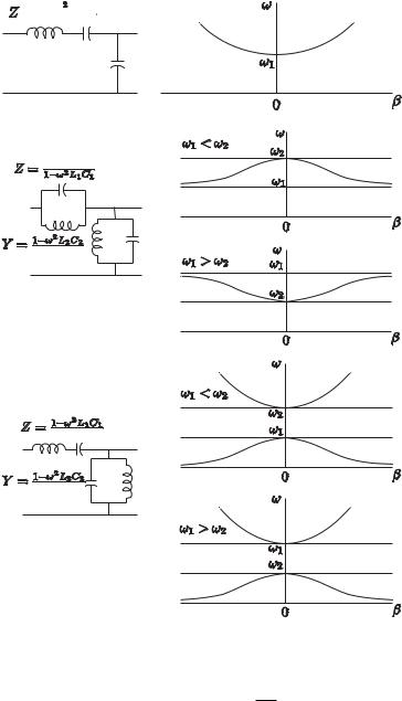
Figure 6.4 A SW structures composed with C and L, with β–ω diagram [after 4].
the line length L, it takes a longer path than that of the antenna (the linear length L0 (Figure 6.3)). Consequently, the wave travel time on the antenna structure of the length L0 becomes equivalently tp which is excess time beyond the travelling time t0 on the length L0. Thus, the phase velocity vp = L0/tp of the wave on the antenna structure is smaller than c = L0/t0, implying that the wave propagates more slowly on the antenna structure corresponding equivalently to the SW.
These wired SW structures are advantageous in designing a small antenna, since a self-resonance condition is easily attained, even though the antenna dimensions are small. In small antennas, self-resonance is significant, because it helps mitigate the matching difficulty in a small antenna arising from its impedance, which is a very low resistive component and a very large reactive component that may combine to produce a large loss and degrade the antenna performance. The wired SW structures have additional advantages; they are fabricated rather simply, with low cost, and can be constructed in planar form, which is very useful for small equipment such as small handsets, handy mobile terminals, and so forth.
The SW structures can be composed with transmission lines, on which impedance components or equivalent boundaries are loaded periodically. The loaded impedances are treated as ordinary lumped components. Examples are shown in Figure 6.4, in which
46 |
Principles and techniques for making antennas small |
|
|
(a) 


 jωC1
jωC1

 jωC2
jωC2
(b)
jωL1
jωL2
(c)
jωC1
jωL2
Figure 6.5 Examples of SW structures: (a), (b), and (c) circuits with β–ω diagrams [4].
one segment of the unit length with β–ω diagrams for each circuit is illustrated [4].
√
Here the propagation constant γ = α + jβ = ZY , where α is the attenuation constant, β is the phase constant, Z is the series impedance per unit length, and Y is the shunt admittance per unit length. In the figure, the dotted line indicates ±kc, below which β is greater than k (the wave number in free space), meaning that vp is smaller than c and so the media supports the SW. The SW structure can be composed by setting appropriate impedances on the transmission line to make β greater than k. Other examples of LC circuits that possibly realize SW structure are illustrated in Figure 6.5 (a), (b) and (c) with
6.2 Techniques and methods for producing ESA |
47 |
|
|
|
|
ω |
|
LR / 2 2CL |
2CL LR / 2 |
|
|
|
|
ωG2 |
|
|
CR |
|
ωG1 |
LL |
|
|
|
|
|
|
|
|
−π |
β |
π |
|
(a) |
(b) |
|
Figure 6.6 (a) An example of equivalent circuit to represent metamaterial and (b) β–ω diagram [6].
μ1 , ε 1
Figure 6.7 A SW structure with dielectric sheet.
Figure 6.8 A SW structure with corrugated surface.
Figure 6.9 A SW structure with trough on the surface.
the β–ω diagrams [5]. The circuits shown in Figure 6.5 can be utilized as metamaterials exhibiting negative phase constant –β by referring to the β − w diagram.
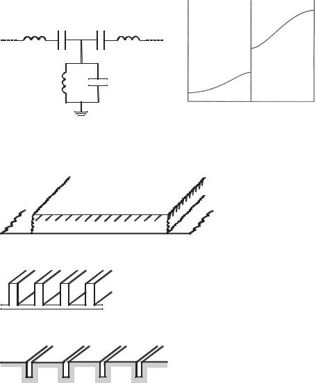
Transmission lines can also be applied to implement metamaterials performance exhibiting either negative ε or negative μ, or both by setting up impedance components appropriately [6]. Examples are shown in Figure 6.6. Applications of this technique to small antennas will be described in later sections.
Two-dimensional SW structures can be made with a dielectric sheet (Figure 6.7), corrugation (Figure 6.8), holey plate, and troughs on the surface (Figure 6.9) [7]. The SW structures can be formed in two-dimensional (2D) structures with transmission lines

48 |
|
|
Principles and techniques for making antennas small |
|||||
|
|
|
|
|
|
|
|
|
|
|
|
|
|
|
|
|
|
|
|
|
|
|
|
|
|
|
|
|
|
|
|
|
|
|
|
|
|
|
|
|
|
|
|
|
0
d
(a) |
(b) |
Figure 6.10 A 2D metamaterial structure composed with transmission line; (a) equivalent circuit [17], (b) practical model [8].
w
=
2L N
3
2
1
a
b
(a) |
(b) |
Figure 6.11 Meander line antenna: (a) antenna structure and (b) an equivalent expression [10].
(Figure 6.10) [8]. Three-dimensional (3D) structure is also composed with transmission lines or bulk materials [9].
6.2.1.1.1.1 Meander line antennas
A meander line may be used as a typical antenna element for reducing the size, as it has the SW structure [10–12]. Applicable antenna types are not only dipoles, but also monopoles over a ground plane, and arrays. The antenna element can be made of thin wire and thin tape printed on the surface of dielectric structure. The performance of a meander line antenna (Figure 6.11(a)) can be found by treating the antenna structure as a series connection of a shorted two-wire transmission line plus a linear element as shown in Figure 6.11(b) [10]. However, the antenna is practically designed by using an electromagnetic simulator, for instance, MoM (Method of Moment) and FDTD (FiniteDifference Time-Domain) [11]. The simulation is simple and yet provides better results as compared with the calculation that uses the equivalent transmission line.
The phase velocity vp of an EM wave on the meander line is approximately given by
(L p/L0)c |
(6.1) |
6.2 Techniques and methods for producing ESA |
49 |
|
|
N
w/λ
Figure 6.12 Relationship between the number of segment N and the width w/λ [after 10].
1.4 |
|
|
|
|
|
1.2 |
|
|
|
|
|
f |
|
|
|
|
|
1 |
|
|
|
|
|
f0 |
|
|
|
|
|
0.8 |
|
|
|
|
|
|
|
|
|
Measured |
|
0.6 |
|
|
|
Calculated |
|
0 |
0.2 |
0.4 |
0.6 |
0.8 |
1 |
|
|
|
b |
|
|
|
|
|
a |
|
|
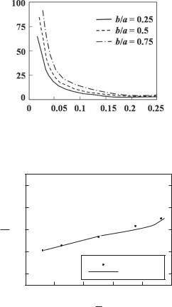
Figure 6.13 Resonance frequency (f/f0) dependence on the ratio of the pitch b/a [10].
where Lp denotes the length of the meandered line and L0 is the length of the linear part of the line.
The resonance frequency f0 is determined mainly by the total length L0 of the line, but in a strict sense it depends on the structural parameters of antennas (the straight length L, width w, pitch a, element width b, and number of equivalent transmission lines N). With the equivalent transmission line model, the resonance wavelength λ0 = c/f0 is given in conjunction with N, which is given by
N = [λ/4 log(2λ/b) − L log(8L/b)]/{w log(2L/N b)[1 + 1/3(βw/2)2]}. (6.2)
This is a transcendental equation which can’t be solved analytically but only numerically and given graphically as shown by Figure 6.12 and Figure 6.13, respectively, where relationships between N and w/λ, and b/a against f/f0 are illustrated. The resonance frequency f0 can be calculated from λ0 and also read from Figure 6.13.
50 |
Principles and techniques for making antennas small |
|
|
[%] 100.0 |
|
|
|
|
|
80.0 |
|
|
|
b/a = 0.25 |
100 |
|
|
|
|
|
|
60.0 |
|
|
|
Exp’t |
|
|
|
|
b/a = 0.50 |
|
|
η |
|
|
|
Exp’t |
N |
40.0 |
|
|
|
b/a = 0.75 |
50 |
|
|
|
|
Exp’t |
|
20.0 |
|
|
|
|
|
0.0 |
0.1 |
0.2 |
0.3 |
0.4 |
0 |
0.0 |
0.5 |
2L
λ
Figure 6.14 Relationship between radiation efficiency η and the length 2L/λ (w/λ = 0.03) [10].
L |
|
|
2L λ (w λ = 0.03) |
|
2a |
|
2.0 |
|
|
|
|
|
|
|
|
k |
cotψ |
|
|
P |
β |
|
|
|
P |
1.0 |
|
|
|
(tanψ = |
|
|
||
2π a) |
0 |
ka cot ψ |
5 |
|
(a) |
|
|
(b) |
|
Figure 6.15 NMHA; (a) antenna structure and (b) relationship between the phase velocity vp and the pitch angle ψ in NMHA [14].
Efficiency η of a meander line antenna is given by using antenna parameters as follows:
η = 1/[1 + 1/4π (Rs/Rd)(λ/b)(N w/L)]. |
(6.3) |
The radiation efficiency η is drawn with respect to b/a as Figure 6.14 shows.
The efficiency of a meander line antenna is lower than that of a linear antenna of length L0 because it has greater loss owing to longer length Lp than the linear antenna of the length L.
Design of this type of antenna will be introduced in Chapter 7.
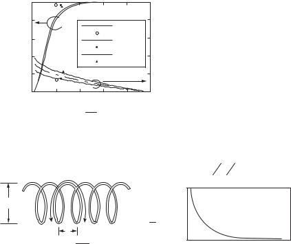
6.2.1.1.1.2 Helical antennas
Here the helical antenna is taken only for the case where radiation is in the direction normal to the antenna axis; that is, Normal Mode Helical Antenna (NMHA) [13]. In the case of NMHA, the phase velocity vp is given approximately by [14]
vp = c sin ψ |
(6.4) |
where ψ is the pitch angle (Figure 6.15).
6.2 Techniques and methods for producing ESA |
51 |
|
|
notch slot
slot
L0 |
L0 |
Figure 6.16 An example of extension of the current path on an antenna structure with a slot and notch.
The resonance frequency depends on the antenna parameters such as the diameter d, pitch angle ψ , and the total length L; however, since it is hardly given analytically, practical design depends on either simulation or approximation.
Practical design methods will be discussed in Chapter 7.
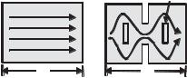
6.2.1.1.1.3 Waveguide structures
Planar surface waveguides propagate either fast or slow waves, depending on the structural parameters of the guides. Usually, these guides are used as relatively large, twodimensional, flush mounted antennas; however, here only SW structures and those applicable to construct small antennas will be taken into consideration. Typical surface guides are planar dielectric sheet (Figure 6.7), holey plate structure, inductive guide structure, corrugated surface (Figure 6.8), capacitive guided structure, and so forth [1, 4].
These guides are not necessarily used as a radiating element, but applied to lowering resonance frequency by placement on a planar antenna surface.
This concept is adopted when equivalent metamaterial performance is required.
6.2.1.1.2 Modification of antenna geometry to extend the current path
The SW structures can be produced by modifying an antenna geometry such that the current flow path is lengthened, resulting in the phase velocity vp equivalently smaller than c in free space, and hence lowering the resonance frequency. A planar antenna, on which a slot or a notch is placed to lengthen the current path so that the electrical size is shortened as shown in Figure 6.16, is an example. In the figure, the direction of the current flow is illustrated with arrows.
The phase velocity vp of the wave travelling on this surface is modified by lengthening the current path L0 to Lp and is approximately given by
vp = (L0/L p)c |
(6.5) |
where Lp is the length of the current path with the slot and L0 is the length without the slot. The resonant frequency is determined approximately by the length Lp.
Multiband operation can be realized by using several slots on a planar structure, by which the current flows on several paths, as shown in Figure 6.17. In this case, each resonance frequency corresponds to one length of the current path.