7.2.5.1Applications of SNG (Single Negative) materials

ε2, μ2 ε1, μ1

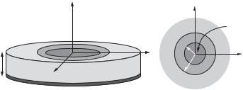
Figure 7.210 Geometry of a circular patch antenna loaded with an MNG MM [112a and b].

with their location, arrangement, and alignment, are shown. To realize the MNG MM, multiple spiral ring resonators (MSRR) (Figure 7.209(c)) are employed as an appropriate selection, having the dimensions that fit with the limited thickness of the space between the patch and the ground plane, while their required resonance frequency is kept despite their small electrical size. The MSRR are aligned according to the expected preferred direction of the magnetic field at their location. Geometry of the patch antenna loaded with an MNG MM is illustrated in Figure 7.210, showing (a) the 3D view and (b) the top view of the antenna, which is partially loaded with an MNG MM underneath the patch. With this arrangement, resonant modes can be excited on the patch, even though the dimensions are significantly smaller than the operating wavelength. Even with the small dimensions, the MNG MM must provide an effective negative permeability in its complex near-field interaction with the feed and the patch. As the MNG MM has dispersion property, the permeability μ1 is given by assuming the Drude dispersion relation as

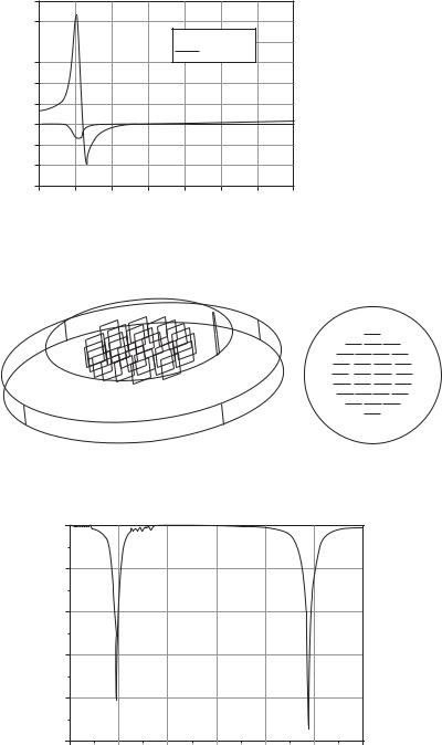
where μ0 is the free space permeability, ωp is the magnetic plasma frequency, and δ is the damping factor. Here the MNG media required to design an antenna shown in Figure 7.210 for operating at 0.47 GHz is assumed to have the dispersion characteristic as shown in Figure 7.211, where the variation of the relative permeability μ1/μ0 with respect to the frequency is given [112a]. In this case, the geometrical parameters of the antenna used are: radius of the substrate a = 20 mm, radius of the MNG media a1 = 12 mm, thickness of the substrate d = 5 mm, and δ = 0.01 GHz. Then the required value of the relative permeability Re[μ1/μ0] = –2.17 at 0.47 GHz. Geometrical sketch of the MNG integrated patch is depicted in Figure 7.212(a). In the figure, (b) illustrates arrangement of the MSR (Multiple Split Ring), viewing from the top of the patch. With this MSR arrangement, almost uniform field distributions are obtained, thus exciting the desired TM11 mode effectively all over the patch. The presence of the MSR highly affects the current distributions underneath the patch, closing itself in an electrically small resonant loop, which produces the desired radiation patterns and gain [112a]. The return-loss characteristic is depicted in Figure 7.213, which shows matching features of the antenna at two frequencies. The antenna operates at higher frequencies (around 2.44 GHz, determined by the electrical size of the patch) as well as lower frequencies. At higher frequencies, the substrate behaves as a homogeneous material having the

Figure 7.214 Geometry of an elliptical patch antenna partially loaded with an MNG MM core surrounded by a DPS shell ([113], copyright C 2010 IEEE).

constitutive parameters ε = ε2 = 2.33 ε0 and μ = μ2 = μ0. The simulated resonance frequencies obtained by using the full-wave commercial code CST Microwave Studio are very close to the predictions using the theoretical cavity model, where the radius of the circular patch antenna is only 20 mm. Radiation patterns are nearly the same as that of an ordinary circular patch antenna. The ground plane in this model has a radius of 40 mm. Simulated gains and efficiencies at the two resonance frequencies, 0.47 GHz and 2.44 GH respectively, are 3.1 dBi, 6.3 dBi and 0.67, 0.92.

7.2.5.1.1.2 Elliptical patch antenna

An elliptical patch antenna loaded with MNG material was studied and showed the possibility of miniaturization of the antenna size and advantages of using the elliptical geometry compared to the use of circular geometry [113]. The antenna geometry is illustrated in Figure 7.214, which shows an elliptically shaped MNG material core of semi-axes a1 and b1 partially loaded underneath the elliptical patch and surrounded by an elliptically shaped DPS shell of semi-axes a2 and b2. The elliptical shape parameters are

the semi-focal length F = a12 − b12 = a22 − b22, and the eccentricity of the elliptical

patch e = 1 − (b2/a2)2 = 1/cosh(ξ 2)(0 ≤ e < 1). Here the Cartesian coordinates x and y are related with the elliptical system coordinates ξ and η by

x = F cos ξ cos η

(7.73)

y = F sin ξ sin η.

Another parameter is the filling ratio Г = (volume of the material core)/(overall volume underneath the patch) (0 < Г < 1).

Based on the full-wave simulation, the antenna performances are analyzed. The parameters used are: surface area of the patch A = 4π cm2, Г = 0.35, e = 0.7, ε1 = ε2 = ε0, and μ2 = μ0. Here, ε1, μ1, and ε2, μ2, respectively, are the constitutive parameters of the MNG and the DPS materials. Since the material has dispersive characteristic, different modes can be excited by the different set of magnetic plasma frequencies. By the selection of ωmp = 1.286 GHz, the odd mode is excited around the design frequency 0.5 GHz, while by the selection of ωmp = 0.707 GHz, the even mode at the same resonance frequency is excited. Simulated return loss S11 is given in Figure 7.215, which indicates that near the design frequency, resonances are obtained in two cases with even and odd mode properties. In the figure, dual-band effect is observed in the odd-mode