Frequency (MHz)

Figure 7.47 Gain characteristics of a MLA shown in Figure 7.6 ([5], copyright C 2006 IEICE).

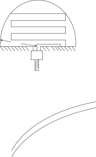
Figure 7.49 illustrates another example; a monopole-type MLA driven by a small loop. Figure 7.50 shows the relative bandwidth with respect to the antenna size kr. Here, r is the radius of a sphere circumscribing the antenna structure and the bandwidth is shown for cases 1/Q and 2/Q. This antenna has appreciably wide bandwidth; for instance, the relative bandwidth is evaluated to be about 10%, although the size kr = 0.5.

There are many other MLAs applied practically to small equipment such as mobile phones. Discussions on these antennas will be provided in later chapters.

7.2.1.1.1.2 Zigzag antennas

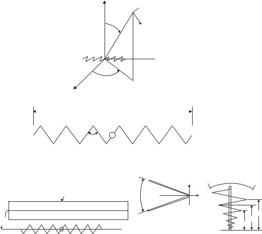
A zigzag antenna composed of a line with alternating salient and re-entrant angles is depicted in Figure 7.51. The zigzag line is formed either uniformly or log-periodically. Since the zigzag line carries a slow wave (SW) with smaller phase velocity than that of free space, the antenna size can be made small. Study of zigzag antennas should go back to a paper published in 1960 [15], in which operation of typical logarithmically periodic zigzag antennas based on near-field measurement had been discussed. Later, other papers treating balanced backfire zigzag antennas [16], theory [17], input impedance [1], and analysis [18], which facilitated antenna design, were published. In [18] two types of zigzag antenna are described; one is a uniform balanced zigzag antenna over a ground plane, and another is a balanced log-periodic zigzag antenna as Figure 7.52 shows. Input impedance of a zigzag dipole antenna is depicted in Figure 7.53, where input impedance of a linear dipole antenna is shown as a comparison. Current distributions on the antenna element are calculated by solving integral equations for antennas, and the numerical results are illustrated in Figure 7.54, where (a) depicts that of the uniform zigzag antenna and (b) the log-periodic zigzag antenna. A k–β diagram is shown in Figure 7.55, where the wire diameter d of the antenna is 0.008λ and two cases in tooth angle, 20 degrees and 30 degrees, are shown.

Figure 7.48 Radiation patterns of an MLA shown in Figure 7.6: (a) and (b) depict radiation patterns on the azimuth plane and the elevation plane, respectively, for antenna on the front side, and (c) and (d) show those on the azimuth plane and the elevation plane, respectively, for antenna on the back side ([5], copyright C 2006 IEICE).

r

Figure 7.49 A meander line monopole antenna driven by a small loop ([6], copyright C 2003

Antenna size (kr)

Figure 7.50 Relative bandwidth of the antenna shown in Figure 7.49 ([6], copyright C 2003 IEEE).

7.2.1.1.1.3 Normal mode helical antennas (NMHA)

The NMHA (Figure 7.56) has been used practically in various small wireless terminals like mobile phones, as it can be produced in small size, and yet with higher radiation efficiency than other types of antennas having the same size. Radiation pattern is essentially the same as that of a linear dipole, and the most significant feature of the NMHA may be in the antenna structure, with which self-resonance can easily be attained, even though the size is small. Self-resonance is favorable for obtaining higher radiation efficiency, because a reactance component, which typically gives rise to a matching-network loss,

l = NL

d

l = 0

Figure 7.56 An NMHA model ([21], copyright C 2008 IEICE).

Study on NMHA has progressed as requirements for small antennas such as the NMHA have increased. Various types of NMHAs such as dielectric-loaded NMHA [21], in which efficient numerical calculation is demonstrated, log-periodic NMHA [22], folded NMHA [23], and two-wire NMHA [24], have so far been used.

Here analysis and design of the NMHA will be briefly introduced by quoting the analysis described in [19–21], and providing design data based on the analysis. The antenna model used for the analysis is shown in Figure 7.57 with the coordinate systems and antenna parameters such as helix radius a, wire diameter d, pitch of helical winding

p

y

Figure 7.57 NMHA model used for the analysis with the coordinate systems [19].

2a

p

( 0 = √(2πa)2 + p2)

Figure 7.58 A segment consisting of two whole turns of helical structure [19].

p, helix one-turn length 0 = (2aπ )2 + p2, and number of helix windings N. The integral equation with respect to the current distribution J ( ) on the wire is

Here V is the feed voltage, δ is a gap at the feed terminal, k = ω√μ0ε0 = 2π/λ stands for phase constant in free space, and r is distance between two points on , and . In order to transform the derivative of Green’s function to that of current functions and to ease solving the integral equation, the Galerkin method will be adopted along with a weighting function, which is zero at the end of the segment. The antenna model is divided into (2N – 1) segments. A segment consists of two whole turns of helical structure taken at an arbitrary place on the antenna, which has length of 2 as shown in Figure 7.58. Then, at the mth segment is described as (m – 1) L ≤ ≤ (m + 1) L, where m takes the values 1, 2, . . . , (2N − 1), and the current Jm( ) on the mth segment is expressed by Im times f ( ), which is a function having the maximum value unity at = mL, and zero

Squared_cosinusoidal

1

0.8

0.6

0.4

0.2

x

Figure 7.59 A squared cosine function ([21], copyright C 2008 IEICE).

at = (m ± 1)L. Here, Im is an unknown coefficient to be determined. Then the current on the antenna J ( ) is given by

m=1

Im can be determined by using the circuit equation

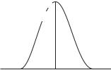
Now a function f ( ), a squared cosine function (Figure 7.59) is selected to give a good approximation as follows

Through some tedious manipulations, constitutional parameters of the NMHA at resonance are analyzed [21]. In the analysis, antenna parameters of relative helix radius a/λ and relative pitch p/λ with respect to the wavelength are taken into consideration and divided into two groups A and B depending on the size. In group A, both a/λ and relative pitch p/λ are relatively larger, lying between 10−3 10−4, and in group B, they are relatively smaller with a/λ between 5 × 10−4 10−3, and p/λ between 10−4 5 × 10−4. Number of turns N at the resonance condition is expressed by illustrating the relationship between a/λ and p/λ in Figure 7.60 for the group A and in Figure 7.61 for the group B, respectively.