- •Contents
- •Preface
- •Chapter 1 Introduction (K. Fujimoto)
- •Chapter 2 Small antennas (K. Fujimoto)
- •Chapter 3 Properties of small antennas (K. Fujimoto and Y. Kim)
- •Chapter 4 Fundamental limitation of small antennas (K. Fujimoto)
- •Chapter 5 Subjects related with small antennas (K. Fujimoto)
- •Chapter 6 Principles and techniques for making antennas small (H. Morishita and K. Fujimoto)
- •Chapter 7 Design and practice of small antennas I (K. Fujimoto)
- •Chapter 8 Design and practice of small antennas II (K. Fujimoto)
- •Chapter 9 Evaluation of small antenna performance (H. Morishita)
- •Chapter 10 Electromagnetic simulation (H. Morishita and Y. Kim)
- •Chapter 11 Glossary (K. Fujimoto and N. T. Hung)
- •Acknowledgements
- •1 Introduction
- •2 Small antennas
- •3 Properties of small antennas
- •3.1 Performance of small antennas
- •3.1.1 Input impedance
- •3.1.4 Gain
- •3.2 Importance of impedance matching in small antennas
- •3.3 Problems of environmental effect in small antennas
- •4 Fundamental limitations of small antennas
- •4.1 Fundamental limitations
- •4.2 Brief review of some typical work on small antennas
- •5 Subjects related with small antennas
- •5.1 Major subjects and topics
- •5.1.1 Investigation of fundamentals of small antennas
- •5.1.2 Realization of small antennas
- •5.2 Practical design problems
- •5.3 General topics
- •6 Principles and techniques for making antennas small
- •6.1 Principles for making antennas small
- •6.2 Techniques and methods for producing ESA
- •6.2.1 Lowering the antenna resonance frequency
- •6.2.1.1 SW structure
- •6.2.1.1.1 Periodic structures
- •6.2.1.1.3 Material loading on an antenna structure
- •6.2.2 Full use of volume/space circumscribing antenna
- •6.2.3 Arrangement of current distributions uniformly
- •6.2.4 Increase of radiation modes
- •6.2.4.2 Use of conjugate structure
- •6.2.4.3 Compose with different types of antennas
- •6.2.5 Applications of metamaterials to make antennas small
- •6.2.5.1 Application of SNG to small antennas
- •6.2.5.1.1 Matching in space
- •6.2.5.1.2 Matching at the load terminals
- •6.2.5.2 DNG applications
- •6.3 Techniques and methods to produce FSA
- •6.3.1 FSA composed by integration of components
- •6.3.2 FSA composed by integration of functions
- •6.3.3 FSA of composite structure
- •6.4 Techniques and methods for producing PCSA
- •6.4.2 PCSA employing a high impedance surface
- •6.5 Techniques and methods for making PSA
- •6.5.2 Simple PSA
- •6.6 Optimization techniques
- •6.6.1 Genetic algorithm
- •6.6.2 Particle swarm optimization
- •6.6.3 Topology optimization
- •6.6.4 Volumetric material optimization
- •6.6.5 Practice of optimization
- •6.6.5.1 Outline of particle swarm optimization
- •6.6.5.2 PSO application method and result
- •7 Design and practice of small antennas I
- •7.1 Design and practice
- •7.2 Design and practice of ESA
- •7.2.1 Lowering the resonance frequency
- •7.2.1.1 Use of slow wave structure
- •7.2.1.1.1 Periodic structure
- •7.2.1.1.1.1 Meander line antennas (MLA)
- •7.2.1.1.1.1.1 Dipole-type meander line antenna
- •7.2.1.1.1.1.2 Monopole-type meander line antenna
- •7.2.1.1.1.1.3 Folded-type meander line antenna
- •7.2.1.1.1.1.4 Meander line antenna mounted on a rectangular conducting box
- •7.2.1.1.1.1.5 Small meander line antennas of less than 0.1 wavelength [13]
- •7.2.1.1.1.1.6 MLAs of length L = 0.05 λ [13, 14]
- •7.2.1.1.1.2 Zigzag antennas
- •7.2.1.1.1.3 Normal mode helical antennas (NMHA)
- •7.2.1.1.1.4 Discussions on small NMHA and meander line antennas pertaining to the antenna performances
- •7.2.1.2 Extension of current path
- •7.2.2 Full use of volume/space
- •7.2.2.1.1 Meander line
- •7.2.2.1.4 Spiral antennas
- •7.2.2.1.4.1 Equiangular spiral antenna
- •7.2.2.1.4.2 Archimedean spiral antenna
- •7.2.2.1.4.3.2 Gain
- •7.2.2.1.4.4 Radiation patterns
- •7.2.2.1.4.5 Unidirectional pattern
- •7.2.2.1.4.6 Miniaturization of spiral antenna
- •7.2.2.1.4.6.1 Slot spiral antenna
- •7.2.2.1.4.6.2 Spiral antenna loaded with capacitance
- •7.2.2.1.4.6.3 Archimedean spiral antennas
- •7.2.2.1.4.6.4 Spiral antenna loaded with inductance
- •7.2.2.2 Three-dimensional (3D) structure
- •7.2.2.2.1 Koch trees
- •7.2.2.2.2 3D spiral antenna
- •7.2.2.2.3 Spherical helix
- •7.2.2.2.3.1 Folded semi-spherical monopole antennas
- •7.2.2.2.3.2 Spherical dipole antenna
- •7.2.2.2.3.3 Spherical wire antenna
- •7.2.2.2.3.4 Spherical magnetic (TE mode) dipoles
- •7.2.2.2.3.5 Hemispherical helical antenna
- •7.2.3 Uniform current distribution
- •7.2.3.1 Loading techniques
- •7.2.3.1.1 Monopole with top loading
- •7.2.3.1.2 Cross-T-wire top-loaded monopole with four open sleeves
- •7.2.3.1.3 Slot loaded with spiral
- •7.2.4 Increase of excitation mode
- •7.2.4.1.1 L-shaped quasi-self-complementary antenna
- •7.2.4.1.2 H-shaped quasi-self-complementary antenna
- •7.2.4.1.3 A half-circular disk quasi-self-complementary antenna
- •7.2.4.1.4 Sinuous spiral antenna
- •7.2.4.2 Conjugate structure
- •7.2.4.2.1 Electrically small complementary paired antenna
- •7.2.4.2.2 A combined electric-magnetic type antenna
- •7.2.4.3 Composite structure
- •7.2.4.3.1 Slot-monopole hybrid antenna
- •7.2.4.3.2 Spiral-slots loaded with inductive element
- •7.2.5 Applications of metamaterials
- •7.2.5.1 Applications of SNG (Single Negative) materials
- •7.2.5.1.1.2 Elliptical patch antenna
- •7.2.5.1.1.3 Small loop loaded with CLL
- •7.2.5.1.2 Epsilon-Negative Metamaterials (ENG MM)
- •7.2.5.2 Applications of DNG (Double Negative Materials)
- •7.2.5.2.1 Leaky wave antenna [116]
- •7.2.5.2.3 NRI (Negative Refractive Index) TL MM antennas
- •7.2.6 Active circuit applications to impedance matching
- •7.2.6.1 Antenna matching in transmitter/receiver
- •7.2.6.2 Monopole antenna
- •7.2.6.3 Loop and planar antenna
- •7.2.6.4 Microstrip antenna
- •8 Design and practice of small antennas II
- •8.1 FSA (Functionally Small Antennas)
- •8.1.1 Introduction
- •8.1.2 Integration technique
- •8.1.2.1 Enhancement/improvement of antenna performances
- •8.1.2.1.1 Bandwidth enhancement and multiband operation
- •8.1.2.1.1.1.1 E-shaped microstrip antenna
- •8.1.2.1.1.1.2 -shaped microstrip antenna
- •8.1.2.1.1.1.3 H-shaped microstrip antenna
- •8.1.2.1.1.1.4 S-shaped-slot patch antenna
- •8.1.2.1.1.2.1 Microstrip slot antennas
- •8.1.2.1.1.2.2.2 Rectangular patch with square slot
- •8.1.2.1.2.1.1 A printed λ/8 PIFA operating at penta-band
- •8.1.2.1.2.1.2 Bent-monopole penta-band antenna
- •8.1.2.1.2.1.3 Loop antenna with a U-shaped tuning element for hepta-band operation
- •8.1.2.1.2.1.4 Planar printed strip monopole for eight-band operation
- •8.1.2.1.2.2.2 Folded loop antenna
- •8.1.2.1.2.3.2 Monopole UWB antennas
- •8.1.2.1.2.3.2.1 Binomial-curved patch antenna
- •8.1.2.1.2.3.2.2 Spline-shaped antenna
- •8.1.2.1.2.3.3 UWB antennas with slot/slit embedded on the patch surface
- •8.1.2.1.2.3.3.1 A beveled square monopole patch with U-slot
- •8.1.2.1.2.3.3.2 Circular/Elliptical slot UWB antennas
- •8.1.2.1.2.3.3.3 A rectangular monopole patch with a notch and a strip
- •8.1.2.1.2.3.4.1 Pentagon-shape microstrip slot antenna
- •8.1.2.1.2.3.4.2 Sectorial loop antenna (SLA)
- •8.1.3 Integration of functions into antenna
- •8.2 Design and practice of PCSA (Physically Constrained Small Antennas)
- •8.2.2 Application of HIS (High Impedance Surface)
- •8.2.3 Applications of EBG (Electromagnetic Band Gap)
- •8.2.3.1 Miniaturization
- •8.2.3.2 Enhancement of gain
- •8.2.3.3 Enhancement of bandwidth
- •8.2.3.4 Reduction of mutual coupling
- •8.2.4 Application of DGS (Defected Ground Surface)
- •8.2.4.2 Multiband circular disk monopole patch antenna
- •8.2.5 Application of DBE (Degenerated Band Edge) structure
- •8.3 Design and practice of PSA (Physically Small Antennas)
- •8.3.1 Small antennas for radio watch/clock systems
- •8.3.2 Small antennas for RFID
- •8.3.2.1 Dipole and monopole types
- •8.3.2.3 Slot type antennas
- •8.3.2.4 Loop antenna
- •Appendix I
- •Appendix II
- •References
- •9 Evaluation of small antenna performance
- •9.1 General
- •9.2 Practical method of measurement
- •9.2.1 Measurement by using a coaxial cable
- •9.2.2 Method of measurement by using small oscillator
- •9.2.3 Method of measurement by using optical system
- •9.3 Practice of measurement
- •9.3.1 Input impedance and bandwidth
- •9.3.2 Radiation patterns and gain
- •10 Electromagnetic simulation
- •10.1 Concept of electromagnetic simulation
- •10.2 Typical electromagnetic simulators for small antennas
- •10.3 Example (balanced antennas for mobile handsets)
- •10.3.2 Antenna structure
- •10.3.3 Analytical results
- •10.3.4 Simulation for characteristics of a folded loop antenna in the vicinity of human head and hand
- •10.3.4.1 Structure of human head and hand
- •10.3.4.2 Analytical results
- •11 Glossary
- •11.1 Catalog of small antennas
- •11.2 List of small antennas
- •Index
164Design and practice of small antennas I
wavelength. Equation (7.65) indicates that the spiral radiates with a constant gain of π in free space. However, all three gains have a periodic ripple with period of approximately 2.2 GHz, which is the inverse of time delay td = 0.45 ns that is caused in the radiated field by the wave travelling on the spiral surface. This arises because of the truncation of the spiral, which is 12 cm from the feed. The time delay which causes ripple tends to be approximately R/c, where R is the radius of the spiral and c is velocity of light in free space.
7.2.2.1.4.4 Radiation patterns
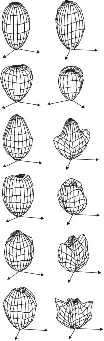
Radiation patterns of the spiral antenna shown in Figure 7.114 (εr = 4.2) are illustrated in Figure 7.120 [49], where only upper hemisphere patterns are given, as the lower hemisphere patterns are the same. The patterns are seen to have alternative contraction and expansion along the z-axis that corresponds to the maxima of the gain ripple. In the dielectric case, it becomes further complicated as the frequency becomes higher, because of deflection of radiated power into side lobes.
7.2.2.1.4.5 Unidirectional pattern
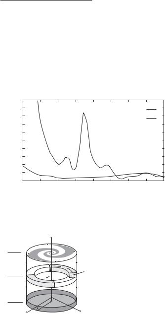
In many practical spiral antenna applications, a unidirectional pattern is required. For this purpose, a conducting shallow cavity is placed behind a spiral antenna. However, since simple use of such a cavity deteriorates the inherent wideband property of the spiral antenna, an absorber may be applied to the outer spiral arms to restore the wideband property [50]. The absorber will suppress reflection of waves caused by the truncation of outer spiral arms. Figure 7.121 illustrates an example of an equiangular spiral antenna, to which a ring-shaped absorber (R-ABS) is applied. In the figure, (a) shows an exploded view, (b) the side view, (c) spiral arms, and (d) a magnified view of near the input terminals. Figure 7.122 illustrates the input impedance; (a) Rin (resistance), (b) Xin (reactance) with and without cavity, (c) with R-ABS. The antenna used here is a two-arm equiangular spiral antenna having parameters provided in Table 7.14, which is backed by a conducting cavity of height Hcav (= antenna height), and diameter Dcav. Axial ratios with and without R-ABS are shown in Figure 7.123. As these figures show, fairly wideband characteristics can be seen with use of R-ABS.
The absorber size can be reduced only to cover near the edge of the outer spiral arms so that no or almost no reflection appears at the ends of the outer spiral arms. Figure 7.124 illustrates an example of the use of arc-shaped ABS (A-ABS) [50]. Input impedance Zin (= Rin + jXin) and axial ratio for a case with A-ABS are shown in Figure 7.125(a) and (b), respectively, and radiation patterns are depicted in Figure 7.126, in which (a) and
(b) show with A-ABS, but for the case where ϕarc = 90◦ and 180◦, respectively, and (c) shows without A-ABS (ϕarc = 0◦).
7.2.2.1.4.6 Miniaturization of spiral antenna
Spiral antennas can be miniaturized by lowering phase velocity of the waves travelling on the spiral arms from the feed point. However, since a spiral antenna has an inherently wide bandwidth property, the phase velocity at a single resonance frequency cannot be taken
7.2 Design and practice of ESA |
165 |
|
|
εr = 1 |
εr= 4.2 |
1.78 GHz
2.88 GHz
3.98 GHz
5.18 GHz
6.28 GHz
7.50 GHz
Figure 7.120 Radiation patterns of antenna shown in Figure 7.114 on the upper hemisphere for cases εr = 1 and 4.2 ([49], copyright C 2007 IEEE).
166 |
Design and practice of small antennas I |
|
|
|
|
Z |
|
|
|
|
|
|
|
|
B |
|
A |
|
|
|
|
|
|
|
|
|
|
|
|
|
|
|
|
|
|
|
|
Ring-shaped |
|
|
|
|
|
|
|
|
|
ABS |
|
|
|
Z |
Spiral |
|
|
|
|
(R-ABS) |
|
|
|
~O |
|
|
|
|
|
|
X |
R-ABS |
|
R-ABS Hcav |
|
|
|
O |
|
|
Cavity |
|
O′ |
||
|
|
|
|
t |
|
|
|
||
|
|
O |
|
|
|
|
|
||
|
|
|
|
|
|
|
|
||
|
|
|
|
|
|
|
|
|
|
x |
Hcav |
|
|
y |
|
|
|
Dcav |
|
|
(a) |
|
|
|
|
|
(b) |
|
|
|
|
|
|
|
|
|
|
||
|
|
|
|
|
|
|
y |
|
|
|
|
|
|
y |
|
|
qB |
pB |
|
|
|
ϕend |
|
|
|
|
|
||
|
|
qB |
|
|
|
|
|
||
|
|
|
|
|
|
|
|
|
|
|
|
pA |
rmax |
|
|
a′ |
τ B |
x |
|
|
|
A |
|
A |
|||||
|
|
|
|
B |
x |
|
a |
|
|
|
|
|
|
|
|
|
|
||
|
|
|
|
A |
|
|
|
ϕst |
|
|
|
|
|
|
|
|
|
||
|
|
|
|
B |
|
|
|
|
|
|
|
|
|
|
|
|
|
|
|
|
|
|
qA |
pB |
|
pA |
|
qA |
|
|
|
|
|
|
|
|
|
||
|
|
|
|
(a) |
|
|
(d) |
|
Figure 7.121 Equiangular spiral antenna with a ring-shaped absorber: (a) exploded view, (b) side view, (c) spiral element, and (d) magnified view around the input terminals ([50], copyrightC 2008 IEEE).
(a) |
|
600 |
|
|
|
|
|
|
|
|
|
|
|
|
|
|
|
|
|
|
|
|
|
|
|
|
|
|
|
|
|
|
|
|
|
|
|
|
|
|
|
|
|
|
with a cavity |
|
|
||||||||
|
|
400 |
|
|
|
|
|
|
|
|
|
|
|
|
|
|
|
|
|
|
|||||||
(Ω) |
|
|
|
|
|
|
|
|
|
|
|
|
|
|
|
|
|
without a cavity |
|
|
|||||||
|
|
|
|
|
|
|
|
|
|
|
|
|
|
|
|
|
|
|
|||||||||
|
200 |
|
|
|
|
|
|
|
|
|
|
|
|
|
|
|
|
|
|
|
|
|
|
|
|
|
|
|
|
|
|
|
|
|
|
|
|
|
|
|
|
|
|
|
|
|
|
|
|
|
|
|
|
|
|
in |
0 |
|
|
|
|
|
|
|
|
|
|
|
|
|
|
|
|
|
|
|
|
|
|
|
|
|
|
R |
−200 |
|
|
|
|
|
|
|
|
|
|
|
|
|
|
|
|
|
|
|
|
|
|
|
|
||
|
|
|
|
|
|
|
|
|
|
|
|
|
|
|
|
|
|
|
|
|
|
|
|
|
|||
|
−400 |
|
|
|
|
|
|
|
|
|
|
|
|
|
|
|
|
|
|
|
|
|
|
|
|
|
|
|
|
2 |
3 |
4 |
5 |
6 |
7 |
8 |
9 |
10 |
|||||||||||||||||
|
|
|
|
|
|
|
|
|
|
|
Frequency (GHz) |
|
|
|
|
|
|
|
|
||||||||
|
|
|
|
|
|
|
|
|
|
|
|
|
|
|
|
(c) |
600 |
|
|
|
|
|
|
|
|
||
|
|
|
|
|
|
|
|
|
|
|
|
|
|
|
|
|
|
|
|
|
|
|
|
||||
|
|
|
|
|
|
|
|
|
|
|
|
|
|
|
|
|
400 |
|
|
|
|
|
|
|
|
||
|
|
|
|
|
|
|
|
|
|
|
|
|
|
|
|
(Ω) |
200 |
|
|
|
|
|
|
|
|
||
|
|
|
|
|
|
|
|
|
|
|
|
|
|
|
|
0 |
|
|
|
|
|
|
|
|
|||
|
|
|
|
|
|
|
|
|
|
|
|
|
|
|
|
in |
|
|
|
|
|
|
|
|
|||
|
|
|
|
|
|
|
|
|
|
|
|
|
|
|
|
−200 |
|
|
|
|
|
|
|
|
|||
|
|
|
|
|
|
|
|
|
|
|
|
|
|
|
|
Z |
|
|
|
|
|
|
|
|
|||
|
|
|
|
|
|
|
|
|
|
|
|
|
|
|
|
|
|
|
|
|
|
|
|
|
|||
|
|
|
|
|
|
|
|
|
|
|
|
|
|
|
|
|
−400 |
|
|
|
|
|
|
|
|
||
|
|
|
|
|
|
|
|
|
|
|
|
|
|
|
|
|
|
|
|
|
|
|
|
|
|||
|
|
|
|
|
|
|
|
|
|
|
|
|
|
|
|
|
|
|
|
2 |
3 |
4 |
(b) 600 |
with a cavity |
|
400 |
||
without a cavity |
(Ω) |
200 |
|
|
|
|
|
|
|
|
|
|
|
|
|
|
|
|
|
|
in |
0 |
|
|
|
|
|
|
|
|
X |
−200 |
|
|
|
|
|
|
|
|
|
|
|
|
|
|
|
|
|
|
|
−400 |
|
|
|
|
|
|
|
|
|
2 |
3 |
4 |
5 |
6 |
7 |
8 |
9 |
10 |
|
|
|
|
Frequency (GHz) |
|
|
|
||
|
|
|
with R-ABS |
|
|
|
|
|
|
|
|
without R-ABS (See) |
|
|
|
|
|
||
|
“with a cavity” in (a) and (b) |
|
|
|
|
|
|||
Rin |
|
|
|
|
|
|
|
|
|
|
Xin |
|
|
|
|
|
|
|
|
5 |
6 |
7 |
8 |
9 |
10 |
|
|
|
|
Figure 7.122 Input impedance of equiangular spiral antenna; (a) Rin resistance (b) reactance (dotted line, with cavity and solid line, without cavity), and (c) Rin and Xin with A-ABS ([50], copyright C 2008 IEEE).
7.2 Design and practice of ESA |
167 |
|
|
Table 7.14 Geometrical parameters ([50], copyright C 2008 IEEE)
symbol |
value |
unit |
|
|
|
r0 |
1.5 |
mm |
as |
0.35 |
rad−1 |
ϕst |
−0.25π |
mm |
ϕend |
2.806π |
rad |
τ |
0.5π |
rad |
Dcav |
120 |
mm |
Hcav |
7 |
mm |
AR (dB)
20 |
|
|
18 |
with R-ABS |
|
|
||
16 |
without R-ABS |
|
14 |
||
|
||
12 |
|
|
10 |
|
|
8 |
|
|
6 |
|
|
4 |
|
|
2 |
|
0
2 |
3 |
4 |
5 |
6 |
7 |
8 |
9 |
10 |
Frequency (GHz)
Figure 7.123 Axial ratio with and without R-ABS ([50], copyright C 2008 IEEE).
|
|
|
Z |
|
|
|
qA |
A |
pA |
(a) |
pB B |
|
||
|
|
qA |
qB |
arc-shaped |
|
|
ϕARC |
||
(b) |
|
t |
|
ABS |
ϕ |
qB |
(ϕ-ABS) |
||
|
|
ARC |
|
|
O |
(c) |
O′ |
x |
y |
Hcav |
Figure 7.124 Equiangular spiral antenna with arc-shaped absorber: (a) spiral element, (b) arc-shaped ABS, and (c) cavity ([50], copyright C 2008 IEEE).
168 |
Design and practice of small antennas I |
|
|
(a) |
600 |
|
|
|
|
|
A-ABSs |
theo. |
|
|
400 |
|
|
|
|
|
|
||
|
|
|
|
|
(ϕARC = 90°){exp |
|
|||
Ω) |
|
|
|
|
Rin |
|
|||
200 |
|
|
|
|
|
|
|
||
( |
|
|
|
|
|
|
|
|
|
in |
|
|
|
|
|
|
|
|
|
Z |
0 |
|
|
|
Xin |
|
|
|
|
|
|
|
|
|
|
|
|
||
|
–200 |
|
|
|
|
|
|
|
|
|
|
|
|
|
|
|
|
|
|
|
–400 2 |
3 |
4 |
5 |
6 |
7 |
8 |
9 |
10 |
Frequency (GHz)
(b) |
10 |
|
|
|
|
A-ABSs |
theo. |
|
|
|
8 |
|
|
|
|
|
|||
(dB) |
6 |
|
|
|
|
(ϕARC = 90°){exp |
|
||
|
|
|
|
|
|
|
|
||
4 |
|
|
|
|
|
|
|
|
|
AR |
|
|
|
|
|
|
|
|
|
2 |
|
|
|
|
|
|
|
|
|
|
|
|
|
|
|
|
|
|
|
|
0 |
3 |
4 |
5 |
6 |
7 |
8 |
9 |
10 |
|
2 |
Frequency (GHz)
Figure 7.125 (a) Input impedance Zin = (Rin + jXin) and (b) axial ratio with A-ABS ([50], copyright C 2008 IEEE).
z |
|
with A-ABSs |
|
with A-ABSs |
|
||
θ |
ϕARC = 90° |
z |
θ |
ϕARC = 180° |
|
||
|
|
|
|||||
0 |
|
|
|
0 |
|
(R-ABS) |
|
−10 |
|
|
|
−10 |
|
|
ER theory |
−20 |
|
|
|
−20 |
|
|
|
|
|
|
|
|
ER expt |
||
−30 |
|
x |
|
−30 |
|
x |
|
[dB] |
|
|
|
[dB] |
|
|
|
(a) |
|
|
|
(b) |
|
|
|
|
|
z |
θ |
without A-ABSs |
|
||
|
|
|
|
||||
|
0 |
|
|
ϕARC = 0° |
|
|
|
|
−10 |
|
|
|
|
|
|
|
−20 |
|
|
|
|
ER |
|
|
−30 |
|
|
x |
|
EL |
|
[dB] |
|
|
|
|
|
|
(c)
Figure 7.126 Radiation patterns; (a) arc = 90◦ , (b) arc = 180◦ , and arc = 0◦ ([50], copyrightC 2008 IEEE).