- •Contents
- •Preface
- •Chapter 1 Introduction (K. Fujimoto)
- •Chapter 2 Small antennas (K. Fujimoto)
- •Chapter 3 Properties of small antennas (K. Fujimoto and Y. Kim)
- •Chapter 4 Fundamental limitation of small antennas (K. Fujimoto)
- •Chapter 5 Subjects related with small antennas (K. Fujimoto)
- •Chapter 6 Principles and techniques for making antennas small (H. Morishita and K. Fujimoto)
- •Chapter 7 Design and practice of small antennas I (K. Fujimoto)
- •Chapter 8 Design and practice of small antennas II (K. Fujimoto)
- •Chapter 9 Evaluation of small antenna performance (H. Morishita)
- •Chapter 10 Electromagnetic simulation (H. Morishita and Y. Kim)
- •Chapter 11 Glossary (K. Fujimoto and N. T. Hung)
- •Acknowledgements
- •1 Introduction
- •2 Small antennas
- •3 Properties of small antennas
- •3.1 Performance of small antennas
- •3.1.1 Input impedance
- •3.1.4 Gain
- •3.2 Importance of impedance matching in small antennas
- •3.3 Problems of environmental effect in small antennas
- •4 Fundamental limitations of small antennas
- •4.1 Fundamental limitations
- •4.2 Brief review of some typical work on small antennas
- •5 Subjects related with small antennas
- •5.1 Major subjects and topics
- •5.1.1 Investigation of fundamentals of small antennas
- •5.1.2 Realization of small antennas
- •5.2 Practical design problems
- •5.3 General topics
- •6 Principles and techniques for making antennas small
- •6.1 Principles for making antennas small
- •6.2 Techniques and methods for producing ESA
- •6.2.1 Lowering the antenna resonance frequency
- •6.2.1.1 SW structure
- •6.2.1.1.1 Periodic structures
- •6.2.1.1.3 Material loading on an antenna structure
- •6.2.2 Full use of volume/space circumscribing antenna
- •6.2.3 Arrangement of current distributions uniformly
- •6.2.4 Increase of radiation modes
- •6.2.4.2 Use of conjugate structure
- •6.2.4.3 Compose with different types of antennas
- •6.2.5 Applications of metamaterials to make antennas small
- •6.2.5.1 Application of SNG to small antennas
- •6.2.5.1.1 Matching in space
- •6.2.5.1.2 Matching at the load terminals
- •6.2.5.2 DNG applications
- •6.3 Techniques and methods to produce FSA
- •6.3.1 FSA composed by integration of components
- •6.3.2 FSA composed by integration of functions
- •6.3.3 FSA of composite structure
- •6.4 Techniques and methods for producing PCSA
- •6.4.2 PCSA employing a high impedance surface
- •6.5 Techniques and methods for making PSA
- •6.5.2 Simple PSA
- •6.6 Optimization techniques
- •6.6.1 Genetic algorithm
- •6.6.2 Particle swarm optimization
- •6.6.3 Topology optimization
- •6.6.4 Volumetric material optimization
- •6.6.5 Practice of optimization
- •6.6.5.1 Outline of particle swarm optimization
- •6.6.5.2 PSO application method and result
- •7 Design and practice of small antennas I
- •7.1 Design and practice
- •7.2 Design and practice of ESA
- •7.2.1 Lowering the resonance frequency
- •7.2.1.1 Use of slow wave structure
- •7.2.1.1.1 Periodic structure
- •7.2.1.1.1.1 Meander line antennas (MLA)
- •7.2.1.1.1.1.1 Dipole-type meander line antenna
- •7.2.1.1.1.1.2 Monopole-type meander line antenna
- •7.2.1.1.1.1.3 Folded-type meander line antenna
- •7.2.1.1.1.1.4 Meander line antenna mounted on a rectangular conducting box
- •7.2.1.1.1.1.5 Small meander line antennas of less than 0.1 wavelength [13]
- •7.2.1.1.1.1.6 MLAs of length L = 0.05 λ [13, 14]
- •7.2.1.1.1.2 Zigzag antennas
- •7.2.1.1.1.3 Normal mode helical antennas (NMHA)
- •7.2.1.1.1.4 Discussions on small NMHA and meander line antennas pertaining to the antenna performances
- •7.2.1.2 Extension of current path
- •7.2.2 Full use of volume/space
- •7.2.2.1.1 Meander line
- •7.2.2.1.4 Spiral antennas
- •7.2.2.1.4.1 Equiangular spiral antenna
- •7.2.2.1.4.2 Archimedean spiral antenna
- •7.2.2.1.4.3.2 Gain
- •7.2.2.1.4.4 Radiation patterns
- •7.2.2.1.4.5 Unidirectional pattern
- •7.2.2.1.4.6 Miniaturization of spiral antenna
- •7.2.2.1.4.6.1 Slot spiral antenna
- •7.2.2.1.4.6.2 Spiral antenna loaded with capacitance
- •7.2.2.1.4.6.3 Archimedean spiral antennas
- •7.2.2.1.4.6.4 Spiral antenna loaded with inductance
- •7.2.2.2 Three-dimensional (3D) structure
- •7.2.2.2.1 Koch trees
- •7.2.2.2.2 3D spiral antenna
- •7.2.2.2.3 Spherical helix
- •7.2.2.2.3.1 Folded semi-spherical monopole antennas
- •7.2.2.2.3.2 Spherical dipole antenna
- •7.2.2.2.3.3 Spherical wire antenna
- •7.2.2.2.3.4 Spherical magnetic (TE mode) dipoles
- •7.2.2.2.3.5 Hemispherical helical antenna
- •7.2.3 Uniform current distribution
- •7.2.3.1 Loading techniques
- •7.2.3.1.1 Monopole with top loading
- •7.2.3.1.2 Cross-T-wire top-loaded monopole with four open sleeves
- •7.2.3.1.3 Slot loaded with spiral
- •7.2.4 Increase of excitation mode
- •7.2.4.1.1 L-shaped quasi-self-complementary antenna
- •7.2.4.1.2 H-shaped quasi-self-complementary antenna
- •7.2.4.1.3 A half-circular disk quasi-self-complementary antenna
- •7.2.4.1.4 Sinuous spiral antenna
- •7.2.4.2 Conjugate structure
- •7.2.4.2.1 Electrically small complementary paired antenna
- •7.2.4.2.2 A combined electric-magnetic type antenna
- •7.2.4.3 Composite structure
- •7.2.4.3.1 Slot-monopole hybrid antenna
- •7.2.4.3.2 Spiral-slots loaded with inductive element
- •7.2.5 Applications of metamaterials
- •7.2.5.1 Applications of SNG (Single Negative) materials
- •7.2.5.1.1.2 Elliptical patch antenna
- •7.2.5.1.1.3 Small loop loaded with CLL
- •7.2.5.1.2 Epsilon-Negative Metamaterials (ENG MM)
- •7.2.5.2 Applications of DNG (Double Negative Materials)
- •7.2.5.2.1 Leaky wave antenna [116]
- •7.2.5.2.3 NRI (Negative Refractive Index) TL MM antennas
- •7.2.6 Active circuit applications to impedance matching
- •7.2.6.1 Antenna matching in transmitter/receiver
- •7.2.6.2 Monopole antenna
- •7.2.6.3 Loop and planar antenna
- •7.2.6.4 Microstrip antenna
- •8 Design and practice of small antennas II
- •8.1 FSA (Functionally Small Antennas)
- •8.1.1 Introduction
- •8.1.2 Integration technique
- •8.1.2.1 Enhancement/improvement of antenna performances
- •8.1.2.1.1 Bandwidth enhancement and multiband operation
- •8.1.2.1.1.1.1 E-shaped microstrip antenna
- •8.1.2.1.1.1.2 -shaped microstrip antenna
- •8.1.2.1.1.1.3 H-shaped microstrip antenna
- •8.1.2.1.1.1.4 S-shaped-slot patch antenna
- •8.1.2.1.1.2.1 Microstrip slot antennas
- •8.1.2.1.1.2.2.2 Rectangular patch with square slot
- •8.1.2.1.2.1.1 A printed λ/8 PIFA operating at penta-band
- •8.1.2.1.2.1.2 Bent-monopole penta-band antenna
- •8.1.2.1.2.1.3 Loop antenna with a U-shaped tuning element for hepta-band operation
- •8.1.2.1.2.1.4 Planar printed strip monopole for eight-band operation
- •8.1.2.1.2.2.2 Folded loop antenna
- •8.1.2.1.2.3.2 Monopole UWB antennas
- •8.1.2.1.2.3.2.1 Binomial-curved patch antenna
- •8.1.2.1.2.3.2.2 Spline-shaped antenna
- •8.1.2.1.2.3.3 UWB antennas with slot/slit embedded on the patch surface
- •8.1.2.1.2.3.3.1 A beveled square monopole patch with U-slot
- •8.1.2.1.2.3.3.2 Circular/Elliptical slot UWB antennas
- •8.1.2.1.2.3.3.3 A rectangular monopole patch with a notch and a strip
- •8.1.2.1.2.3.4.1 Pentagon-shape microstrip slot antenna
- •8.1.2.1.2.3.4.2 Sectorial loop antenna (SLA)
- •8.1.3 Integration of functions into antenna
- •8.2 Design and practice of PCSA (Physically Constrained Small Antennas)
- •8.2.2 Application of HIS (High Impedance Surface)
- •8.2.3 Applications of EBG (Electromagnetic Band Gap)
- •8.2.3.1 Miniaturization
- •8.2.3.2 Enhancement of gain
- •8.2.3.3 Enhancement of bandwidth
- •8.2.3.4 Reduction of mutual coupling
- •8.2.4 Application of DGS (Defected Ground Surface)
- •8.2.4.2 Multiband circular disk monopole patch antenna
- •8.2.5 Application of DBE (Degenerated Band Edge) structure
- •8.3 Design and practice of PSA (Physically Small Antennas)
- •8.3.1 Small antennas for radio watch/clock systems
- •8.3.2 Small antennas for RFID
- •8.3.2.1 Dipole and monopole types
- •8.3.2.3 Slot type antennas
- •8.3.2.4 Loop antenna
- •Appendix I
- •Appendix II
- •References
- •9 Evaluation of small antenna performance
- •9.1 General
- •9.2 Practical method of measurement
- •9.2.1 Measurement by using a coaxial cable
- •9.2.2 Method of measurement by using small oscillator
- •9.2.3 Method of measurement by using optical system
- •9.3 Practice of measurement
- •9.3.1 Input impedance and bandwidth
- •9.3.2 Radiation patterns and gain
- •10 Electromagnetic simulation
- •10.1 Concept of electromagnetic simulation
- •10.2 Typical electromagnetic simulators for small antennas
- •10.3 Example (balanced antennas for mobile handsets)
- •10.3.2 Antenna structure
- •10.3.3 Analytical results
- •10.3.4 Simulation for characteristics of a folded loop antenna in the vicinity of human head and hand
- •10.3.4.1 Structure of human head and hand
- •10.3.4.2 Analytical results
- •11 Glossary
- •11.1 Catalog of small antennas
- •11.2 List of small antennas
- •Index
174 |
Design and practice of small antennas I |
|
|
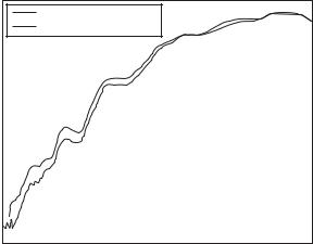
Measured boresight gain (dBic)
5 |
Resistive taper |
|
|
|
|
|
|
0 |
Single chip resistor |
|
|
−5 |
Measured without cavity |
|
|
|
|
|
|
−10 |
|
|
|
−15 |
|
|
|
−20 |
|
|
|
−25 |
|
|
|
−30 |
|
|
|
−35 |
|
|
|
−40 |
1 |
1.5 |
2 |
0.5 |
Frequency (GHz)
Figure 7.134 Measured gain of the 2-inch square spiral antenna with a resistive taper and a single resistor termination ([53], copyright C 2005 IEEE).
This implies 36% size reduction or lowering of the operation frequency for the same size aperture without additional effort to improve impedance matching.
7.2.2.1.4.6.4 Spiral antenna loaded with inductance
Spiral arms are modified to increase their effective length by loading inductance on the arms. Inductive loading on the spiral wire arms can be formed with either planar meandering with rectangular or zigzag, or 3D coiling of the spiral line. Figure 7.136 illustrates a spiral element replaced with (a) planar meander line, and (b) loop-like winding (rectangular or conical) [58]. Gain of the 6-inch spiral antennas is evaluated to compare dependence of the spiral structures such as planar meandering spiral, volumetric spiral, and simple (straight wired) spiral as Figure 7.137 illustrates.
7.2.2.2 Three-dimensional (3D) structure
To improve antenna performance in a small antenna, efficient use of a volume, within which an antenna is contained, is considered. When an antenna takes a three-dimensional (3D) structure, the utmost 3D structure for this purpose is a sphere, and use of the periphery of the sphere is ideal. So far some attempts at placing helical elements on the periphery of a sphere have been made for efficient use of the periphery of a sphere so as to obtain the lower Q compared with other types of antenna having an electrically small size [31].
Other types of structures than spheres are possible to realize small antennas having lower Q in comparison with 2D structures of the same size, if the volume is within the reasonable dimensions for practical use. Typical antennas having such 3D structures are Koch tree, cylindrical helix, cube, and so forth.
7.2 Design and practice of ESA |
175 |
|
|
(a) |
|
|
|
0.6300” |
|
|
|
|
|
|
0.0625” |
|
|
|
|
|
|
|
|
||||||
0.5000” |
|
|
|
|
|
|
||||||
2.6100” |
|
|
|
|
|
|
|
|||||
|
|
|
|
|
|
|
|
|||||
|
|
|
|
|
|
|
|
|
|
|
|
|
|
|
|
|
|
|
|
|
|
|
|
|
|
|
|
|
|
Cross section of tapered superstrate |
|
Loaded 2” spiral |
|
Loaded 6” spiral |
|
(b) 5 |
|
|
|
|
(dBic) |
0 |
|
|
|
−5 |
|
|
|
|
gain |
|
|
|
|
|
|
|
|
|
realized |
−10 |
|
|
|
Measured |
−15 |
ε1 |
= 1 |
|
|
|
|||
|
|
ε1 = 9, thickness = 7.3 mm |
|
|
|
−20 |
ε1 = 16, thickness = 6.1 mm |
|
|
|
ε1 |
= 30, thickness = 4.3 mm |
|
|
|
|
|
||
|
|
ε1 = 90, thickness = 2 mm |
|
|
|
−25 |
|
|
|
|
0.5 |
1 |
1.5 |
2 |
|
|
Frequency (GHz) |
|
Figure 7.135 (a) Cross section of tapered dielectric superstrate placed on the slot spiral and photos, and (b) variation of measured total circularly polarized gain for the 2-inch square spiral antenna depending on various dielectrics ([53], copyright C 2005 IEEE).
Thickness
(a) |
(b) |
Width |
Pitch |
|
|
Figure 7.136 Inductive loading of the 6-inch diameter spiral antennas: (a) with planar meandering and (b) with volumetric coiling ([58], copyright C 2006 IEEE).
176 |
Design and practice of small antennas I |
|
|
Realized total gain (dBic)
5
0
−5
−10
−15
−20
−25
100
Straight wire
Planar meander
Conical coil, tmax = 90 mil
Conical coil, tmax = 250 mil
Conical coil, tmax = 500 mil
200 |
300 |
400 |
500 |
600 |
700 |
800 |
900 |
1000 |
Frequency (MHz)
Figure 7.137 Gain comparison between three types of spiral antennas; ordinary wire spiral, planar meandering, and volumetric coiling ([58], copyright C 2006 IEEE).
Iteration |
0 |
1 |
2 |
3 |
4 |
5 |
Koch dipole
Quasi-fractal tree dipole
3D Quasifractal tree dipole
Figure 7.138 Three types of fractals: Koch dipole, quasi-fractal tree dipole and 3D quasi-fractal tree dipole ([44], copyright C 2002 IEEE).
7.2.2.2.1 Koch trees
Modeling dipoles with Koch Fractal structures are shown in Figure 7.138, where ordinary Koch dipole, quasi-fractal tree dipole, and 3D fractal tree dipole are depicted [44]. In the fractal tree, the top third of every branch is split into two sections and the 3D version has the top third of each branch split into four segments that are each one-third in length. The 3D fractal here implies only that the structure is not contained in a plane.
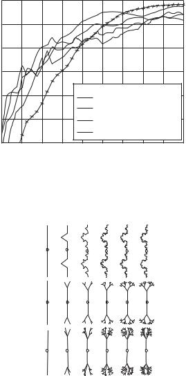
As one way for evaluating the performance, Q of the antenna for each type is compared. Figure 7.139 provides Q of (a) Koch dipole, (b) quasi-fractal tree dipole, and (c) 3D
7.2 Design and practice of ESA |
177 |
|
|
(a)50
45
40 K0 Q
35 K1 Q
30 K2 Q
Q |
25 |
|
|
|
|
|
|
|
|
|
|
K3 Q |
20 |
|
|
|
|
|
|
|
|
|
|
K4 Q |
|
|
|
|
|
|
|
|
|
|
|
|
||
|
15 |
|
|
|
|
|
|
|
|
|
|
K5 Q |
|
10 |
|
|
|
|
|
|
|
|
|
|
|
|
|
|
|
|
|
|
|
|
|
|
Fundamental limit |
|
|
5 |
|
|
|
|
|
|
|
|
|
|
|
|
|
|
|
|
|
|
|
|
|
|
|
|
|
0 |
|
|
|
|
|
|
|
|
|
|
|
|
0.64 |
0.72 |
0.80 |
0.88 |
0.96 |
1.04 |
1.12 |
1.19 |
1.27 |
1.35 |
1.43 |
1.51 |
|
|
|
|
|
|
|
kh |
|
|
|
|
|
(b) |
50 |
|
|
|
|
|
|
|
|
|
|
|
|
45 |
|
|
|
|
|
|
|
|
|
|
K0 Q |
|
40 |
|
|
|
|
|
|
|
|
|
|
|
|
35 |
|
|
|
|
|
|
|
|
|
|
K1 Q |
|
30 |
|
|
|
|
|
|
|
|
|
|
K2 Q |
Q |
25 |
|
|
|
|
|
|
|
|
|
|
K3 Q |
|
20 |
|
|
|
|
|
|
|
|
|
|
K4 Q |
|
15 |
|
|
|
|
|
|
|
|
|
|
|
|
|
|
|
|
|
|
|
|
|
|
K5 Q |
|
|
10 |
|
|
|
|
|
|
|
|
|
|
|
|
|
|
|
|
|
|
|
|
|
|
Fundamental limit |
|
|
5 |
|
|
|
|
|
|
|
|
|
|
|
|
0 |
|
|
|
|
|
|
|
|
|
|
|
0.64 |
0.71 |
0.77 |
0.83 |
0.90 |
0.96 |
1.02 |
1.08 |
1.15 |
1.21 |
1.27 |
1.34 |
1.40 |
1.46 |
1.52 |
|
|
|
|
|
|
|
kh |
|
|
|
|
|
|
|
(c)50
45
40
35
|
30 |
Q |
25 |
|
20 |
15
10
5
0
0.64 |
0.71 |
0.77 |
0.83 |
0.90 |
0.96 |
1.02 |
1.08 |
1.15 |
1.21 |
1.27 |
1.34 |
1.40 |
1.46 |
1.52 |
|
|
|
|
|
|
|
kh |
|
|
|
|
|
|
|
3DT0 Q
3DT1 Q
3DT2 Q
3DT3 Q
3DT4 Q
3DT5 Q
Fundamental limit
Figure 7.139 Comparison of Q between (a) Koch dipole, (b) fractal tree, and (c) 3D fractal tree ([44], copyright C 2002 IEEE).
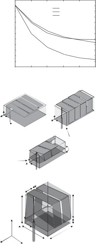
quasi-fractal tree dipole, respectively. The 3D fractal tree shows the lowest Q, and the lowest resonance frequency as shown in Figure 7.140 [45], meaning that this type uses the given space most efficiently.
7.2.2.2.2 3D spiral antenna
A very small spiral antenna to be used for bio-medical telemetry has been developed, and the design and realization of the antenna is introduced [65]. Antenna design started from a planar meander line structure, then its folded structure, and finally progressed to 3D spiral structure as shown in Figure 7.141. Geometry and dimensions of the optimized design of the antenna are shown in Figure 7.142. Reflection factor |S11|
|
2000 |
|
|
|
|
|
|
1900 |
|
|
Koch dipole |
|
|
|
1800 |
|
|
|
|
|
(MHz) |
|
|
Fractal tree dipole |
|
||
1700 |
|
|
3D fractal tree dipole |
|
||
|
|
|
|
|
||
1600 |
|
|
|
|
|
|
frequency |
|
|
|
|
|
|
1500 |
|
|
|
|
|
|
1400 |
|
|
|
|
|
|
1300 |
|
|
|
|
|
|
Resonant |
|
|
|
|
|
|
1200 |
|
|
|
|
|
|
1100 |
|
|
|
|
|
|
1000 |
|
|
|
|
|
|
|
|
|
|
|
|
|
|
900 |
|
|
|
|
|
|
800 |
1 |
2 |
3 |
4 |
5 |
|
0 |
Fractal iteration
Figure 7.140 Computed resonance frequency for three types of fractal dipole as function of the number of iterations ([45], copyright C 2003 IEEE).
Coaxial |
Ground |
|
plane |
||
feeder |
||
|
||
|
Two |
|
Grounding |
substrates |
|
|
||
pin |
|
|
|
Figure 7.141 Design step to develop 3D spiral structure ([65]).
xs = 1
|
xp = 4.5 |
|
|
h = 15 |
hd = 12.75 |
|
|
|
|
z |
|
|
z |
hb = 2.25 |
|
|
|
|
x |
|
|
yg = 14 |
xg = 14 |
x |
y |
|
|
|
Figure 7.142 Geometry and dimensions of the optimized design [65].
7.2 Design and practice of ESA |
179 |
|
|
|
0 |
|
|
|
|
|
|
|
|
|
|
|
|
|
|
|
|
|
|
|
|
|
|
|
|
|
|
|
|
|
|
|
–5 |
|
|
|
|
|
|
|
|
|
|
|
|
|
|
|
|
|
|
|
|
|
|
|
|
|
|
|
|
|
|
|
–10 |
|
|
|
|
|
|
|
|
|
|
|
|
|
|
|
|
|
|
|
|
|
|
|
|
|
|
|
|
|
|
| (dB) |
–15 |
|
|
|
|
|
|
|
|
|
|
|
|
|
|
|
|
|
|
|
|
|
|
|
|
|
|
|
|
||
–20 |
|
|
|
|
|
|
|
|
|
|
|
|
|
|
|
|
|
|
|
|
|
|
|
|
|
|
|
|
|
||
11 |
|
|
|
|
|
|
|
|
|
|
|
|
|
|
|
|S |
–25 |
|
|
|
|
|
|
|
|
|
|
|
|
|
|
|
|
|
|
|
|
|
|
|
|
|
|
|
|
|
|
|
|
|
|
|
|
|
|
|
|
|
|
|
|
|
|
|
–30 |
|
|
|
|
|
|
|
|
|
|
|
|
|
|
|
|
|
|
|
|
|
|
|
|
|
|
|
|
|
|
|
–35 |
|
|
|
|
|
|
|
|
|
|
|
|
|
|
|
|
|
|
|
|
|
|
|
|
|
|
|
|
|
|
|
–40 |
|
|
|
|
|
|
|
|
|
|
|
|
|
|
|
|
|
350 |
400 |
450 |
500 |
|||||||||
|
300 |
Frequency (MHz)
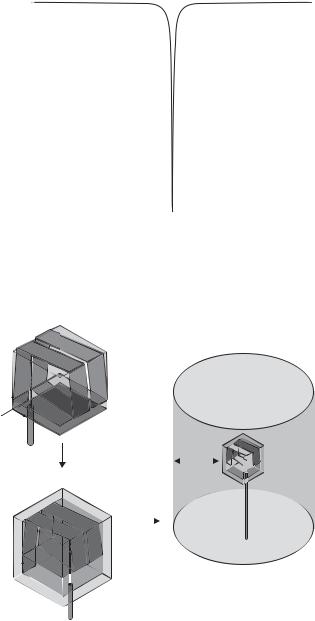
Figure 7.143 S11 performance [65].
Final free space design
Equivalent homogeneous body model
x
Biocompatible insulation
Body thickness
x
Figure 7.144 Introduction of insulation layer to the antenna structure and equivalent model of the body [65].
is illustrated in Figure 7.143. Since the antenna is used in a human body, the antenna element should be insulated to avoid direct contact with the body tissues, and a biocompatible insulator with dielectric constant εr = 3.2 and tan δ = 0.01, is introduced. Figure 7.144 depicts the final free-space design and the biocompatible insulation model. Figure 7.145 illustrates variation of simulated |S11| depending on the thickness of the