1PEC wires; infinite PEC ground plane.

2copper wires; infinite PEC ground plane.

31.5 m circular ground plane.

where γ is an angular separation between two neighbor rings. A prototype SSR antenna is fabricated with Nsr = 17, wire diameter = 1.63 mm, driven dipole length α = 33◦. Simulated input impedance is 43 and the resonance frequency is 403 MHz, which corresponds to the antenna electrical size ka = 0.184. Measured input impedance when the antenna is placed on the ground plane of the radius 1.5 m is 51 . Simulated Q/Qlb is comparable with that of the MSH antenna. Performance parameters of the SSR are given in Table 7.21, where both simulated and measured results are provided.

7.2.2.2.3.5 Hemispherical helical antenna

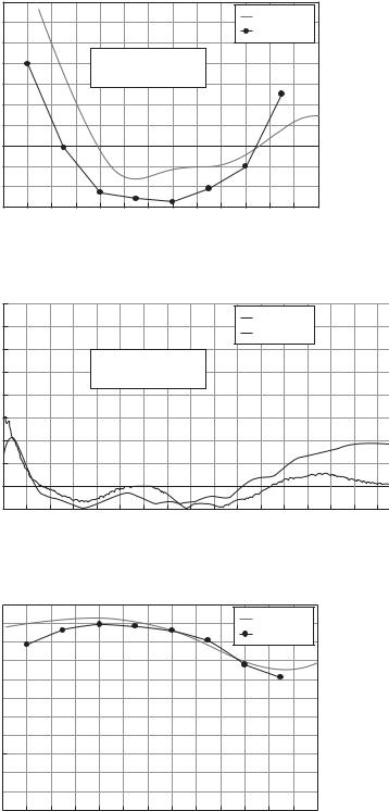
In situations where antennas having compact structure, small size, and yet light weight, are urgently required in aerospace and mobile terminals, use of the hemispherical helix is desirable. New design of the hemispherical helix (HSH) antenna is explored and its wideband performance is introduced in [79]. The antenna is a 4.5 turn HSH with tapered strip radiating element. The width of the tapered element starts with 1 mm and ends with 4 mm, and the hemisphere radius is 20 mm. The antenna is fed at the side with non-linearly tapered matching section, and radiates a circularly polarized wave with wide beam width in the frequency range of 2.2–3.7 GHz. A prototype HSH antenna is constructed and measured for axial ratio, VSWR, and directivity. They are shown in Figure 7.165 through Figure 7. 167 along with simulated results, which have generally good agreement with measured results.

7.2.3Uniform current distribution

7.2.3.1Loading techniques

7.2.3.1.1 Monopole with top loading

The history of top-loaded antennas goes back to 1885, when Edison patented a communication system using a top-loaded antenna [80]. Hertz demonstrated electromagnetic waves in 1888 by using a dipole with large conducting plates attached to each end, which acted as a resonator with an inductance of the high-voltage-generator inductive coil. In the early days of communications, transmission of very low frequency (VLF) bands was accomplished by applying top-loading techniques to short monopoles that were subsequently adapted to LF, MF, and HF communications. In those days, most antennas

Figure 7.165 Measured and simulated axial ratio ([79], copyright C 2010 IEEE).

Figure 7.167 Measured and simulated directivity ([79], copyright C 2010 IEEE).

z

b

2a

h

ϕ

r

Figure 7.168 Cross section of a disk-plate top-loaded monopole mounted on an infinite ground plane ([82], copyright C 2008 IEEE).

could be categorized as electrically small antennas and hence nowadays application of the top-loading technique to produce electrically small antenna is not necessarily new, but rather prevalent.

As an electrically small monopole has small radiation resistance and large capacitive reactance, addition of either a capacitive or inductive component to the monopole is implemented to make self-resonance and matching conditions feasible. Top loading was used as one of the most common means to realize capacitive loading on the monopole [81]. Practical inductive loading has been implemented by coil loading in the middle of a monopole element [82] and by modifying a linear monopole to either a meandered or helical wire structure.

Since top loading is effective to lower the resonance frequency, it is useful for reducing the antenna height and in turn for equivalently increasing the electrical length of a short monopole, assisting improvement of antenna performances. This increases radiation resistance and bandwidth even with the antenna of reduced size. The top loading can be ascribed to producing the uniform current distribution on the short monopole that yields significant improvements described above.

Top loading on a short monopole is implemented by a wire of L-shape (Inverted-L), T-shape, and crossed multi-elements, among others. A thin circular plate (disk) and its variations are also used as another common type of top loading. A circularly symmetric thin planar conductor top loaded on an electrically small monopole placed on the infinite ground plane shown in Figure 7.168 is representative [82]. In practice, the disk can take other forms, as Figure 7.169 illustrates: (a) wire-grid disk, (b) wired spiral, and (c) wiregrid spherical cap [83a, b]. There are of course dipole types as shown in Figure 7.169(d), where the top load is a wire grid, and also the monopole can be a meandered wire, and a helical wire as well. Figure 7.169(e) and (f) show examples of a wire-grid top-loaded helical dipole and a spherical-cap top-loaded helical dipole, respectively [83a, b].

In the planar disk model shown in Figure 7.168, currents on the monopole and the field they produce are treated as independent of the azimuthal angle ϕ. With dimensions h = 0.3 m, b = 0.6 m, and a = 6.35 mm, and the operating frequency f0 = 10 MHz,

Figure 7.169 (a) Wire-grid disk top-loaded monopole, (b) wired-spiral hat top-loaded monopole,

(c) wire-grid spherical-cap top-loaded monopole, (d) wire-grid disk top-loaded dipole,

(e) wire-grid top-loaded helical dipole, and (f) spherical-cap top-loaded helical dipole, ([83a, b], copyright C 2008 IEEE).

current and charge distributions on the monopole and the disk are shown in Figure 7.170 and Figure 7.171, respectively, in which the current on the monopole until h = 0.01λ is observed nearly uniform. The input impedance (= R + jX) is depicted in Figure 7.172, where both calculated and measured results are shown. Radiation power factor pe, radiation conductance Ge, and bandwidth f along with applied voltage V are illustrated as functions of the top-loaded ratio b/h in Figure 7.173 and Figure 7.174, respectively. In these figures, pe0 and Ge0, respectively, denote reference values for an antenna with b = h. The beneficial effect of top-loading is obvious from increases in bandwidth f (proportional to pe), and radiated power (proportional to Ge). Particularly the bandwidth with b/h = 5 is over 250 times as much when compared with that of b/h = 0.02, the unloaded monopole. These figures suggest that top loading is vitally important to reduce the input voltage to a tolerable level and to achieve the required bandwidth.

Another type of top-loaded monopole is an electrically small monopole simply loaded with an open-circuited transmission line shown in Figure 7.175 [84].

The input impedance Z is

Measured

2πh/λ, antenna height in radians

Figure 7.172 Theoretical and measured impedance of a DLM with h = b = 0.3 m, and a = 6.36 mm ([82], copyright C 2008 IEEE).

b/h, top loading ratio

Figure 7.173 Radiation power factor (normalized) pe and radiation conductance Ge as function of b/h for a reference antenna with h = b = 0.3 m, and a = 6.35 mm ([82], copyright C 2008 IEEE).