


158 |
Design and practice of small antennas I |
|
|
(a)
Real (Zin) Ω
(b)
Imag (Zin) Ω
300
Experiment
Simulation
200
100
30
1 |
2 |
4 |
8 |
f (GHz)
Experiment
Simulation
100
0
−100
1 |
2 |
4 |
8 |
f (GHz)
Figure 7.110 Input impedance of a five-order Sierpinsky monopole: (a) real part and (b) imaginary part (solid line: measured, dashed line; simulated by using FDTD, and dashed-dotted line; simulated by using DOTIG4 ([47], copyright C 2003 IEEE).
Input impedances are given in Figure 7.110, where (a) shows resistance and (b) shows reactance.
7.2.2.1.4 Spiral antennas
Antenna performances of dipoles and loops generally depend on the frequency; however, there are some antennas like self-complementary antennas which have frequencyindependent characteristics. Other types, such as spiral antennas also have frequencyindependent characteristics. The antenna structure is essentially determined by angle, not length, with which the antenna exhibits constant impedance characteristics. Ideally the spiral antenna of infinite structure is frequency independent; however, a practical antenna cannot have infinite structure, the frequency dependence on its impedance being limited by the finite structure; that is, the outer length of spiral curve and the impedance becomes constant over the frequency higher than that determined by the outer spiral length. Two types of spiral antenna are representative: equiangular spiral antenna and Archimedean spiral antenna.
7.2.2.1.4.1 Equiangular spiral antenna
The basic equiangular spiral curve shown in Figure 7.111 is expressed by
r = r0eaϕ |
(7.60) |

7.2 Design and practice of ESA |
159 |
|
|
y
r
φ
x
Figure 7.111 Equiangular spiral curve ([48]).
|
δ |
|
|
|
Edge 1 |
|
|
|
|
r1 |
r1 |
|
|
|
R |
|
|
||
r4 |
|
|
|
|
r3 |
|
|
|
|
Edge 2 |
|
|
|
|
(a) |
(b) |
= |
|
|
Figure 7.112 (a) Planar equiangular spiral antenna (self-complementary case with δ |
90◦ ([48]) |
|||
|
||||
and (b) a conical equiangular spiral structure.
where r0 denotes radius for ϕ = 0, and a is a constant controlling the flare rate of the spiral [48]. The spiral in the figure is right-handed, but left-handed spirals can be generated using negative values of a, or simply turning the spiral in the opposite direction. A planar equiangular spiral antenna is created by using the equiangular spiral curve shown in Figure 7.112 (a). Each edge of the spiral element has a curve basically expressed by (7.60). For instance, r1 = r0eaϕ , r2 is the curve rotated through angle δ, so r2 = r0 ea(ϕ –δ ), r3 has the curve of δ = π , then r3 = r0ea(ϕ –π ), and r4 is the curve further turned from r3, so r4 = r0ea(ϕ –π –δ ).
Figure 7.112(b) depicts a conical equiangular spiral structure.
The flare rate a is more conveniently expressed by using expansion factor ε, which is
ε = r(ϕ + 2π )/r(ϕ) = r0ea(ϕ+2π )/r0eaϕ = ea2π . |
(7.61) |
A typical value for ε is 4, and then a = 0.221. The upper frequency fu is determined by the feed structure. The minimum radius r0 is about λ/4 at fu for ε = 4. A nearly

160 |
Design and practice of small antennas I |
||||
|
|
|
|
|
|
|
|
|
|
|
|
|
|
|
|
|
|
|
|
|
|
|
|
|
|
|
|
|
|
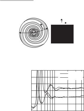
Figure 7.113 (a) A circular type Archimedean spiral antenna and (b) a square type Archimedean spiral structure.
equivalent criterion is a circumference in the feed region of 2π r0 = λu = c/fu. The lowest frequency fL is set by overall radius R, which is roughly λL/4 (λL = c/fL), and the circumference C of a circle, which encloses the entire spiral, is used to set fL by taking C = 2π R = λL. When a = 0.221, R is r(ϕ = 3π ) = r0 e0.221(3π ) = 8.03 r0 and equals λL/4. Meanwhile, r0 equals λu/4, then, the bandwidth defined by λL/λu = 8.03, meaning about 8:1 bandwidth.
7.2.2.1.4.2 Archimedean spiral antenna
Figure 7.113 illustrates the planar Archimedean spiral antenna [48], having two spiral curves, which are linearly proportional to the polar angle rather than exponential for the equiangular spiral, represented by
r = r0(1 + ϕ/π ) and r0(1 + ϕ/π − p). |
(7.62) |
The outside circumference in this case is one wavelength (a half wavelength for the outer half-circle) and an antenna with three turns is shown in Figure 7.113(a). Since the radiated fields produced by the two spirals are orthogonal, equal in magnitude, and 90 degrees phase difference, the wave is left-hand circular polarization (LHCP). The lefthand winding of the spiral determines the left-hand sense in the wave, which is viewed as radiation out of the page, and the opposite sense of wave is viewed as radiation toward the other side of page, that is RHCP.
Figure 7.113(b) illustrates a square Archimedean spiral modified from circular type. The spiral produces a broad main beam perpendicular to the plane of the spiral; however, in many practical applications, a unidirectional beam is preferred. This suggests the use of a ground plane or cavity, over which the spiral is placed. The latter is called a cavity-backed spiral antenna. Since by using metallic material for the cavity, it is natural that the frequency performance is altered, leading to use of absorbing material loaded
into the cavity to reduce the frequency variation.
The typical performance parameters for a cavity-backed Archimedean spiral antenna are HP (Half power beamwidth) = 75◦, |AR| = 1 dB, G = 5 dB over 10:1 bandwidth or more [48]. The input impedance is approximately 120resistive.
Rout
7.2 Design and practice of ESA |
161 |
|
|
|
|
y
z x
x
ψ
R in
in
Figure 7.114
IEEE).
|
300 |
|
(Ω) |
250 |
|
200 |
||
Resistance |
||
150 |
||
|
||
|
100 |
|
|
50 |
|
|
0 |
Geometry of truncated two-arm equiangular spiral antenna ([49], copyright C 2007
Measured
FDTD
εr ≈ 1
εr = 6.15
0.5 |
1 |
2 |
3 |
4 |
Frequency
Figure 7.115 Measured and FDTD simulated resistance for antenna type A and B ([49], copyrightC 2007 IEEE).
7.2.2.1.4.3 Antenna performance and design of spiral antenna 7.2.2.1.4.3.1 Input impedance
A model considered here is depicted in Figure 7.114 [49], which shows major design parameters Rin, Rout, and . Here two cases, A and B, where a spiral element is embedded on two different substrates, are treated. The dimensional parameters (see Fig. 7.114) are Rin = 3 mm, Rout = 0.114 m, = 79◦. The antenna type A uses substrate modeled as a 0.1 mm polyester film layer εr = 3.2 on top of a foam layer εr = 1, while the antenna type B uses substrate modeled as a uniform dielectric with a thickness of 1.27 mm and εr = 6.15. Input impedances measured and calculated by using FDTD simulator are depicted in Figure 7.115, showing resistance, and Figure 7.116(a) and (b), showing reactance for the type A and the type B, respectively. Impedance characteristics tend to show peculiar behavior having three distinct regions. The outer truncation of the spiral curve dominates the performance in low-frequency regions, the inner truncation determines that in higher-frequency behavior, and the shape of the spiral curve itself relates to that of the intermediate-frequency regions. There is a region where a band of nearly constant impedance is seen between the erratic behavior at the upper and lower frequencies. This is the specific behavior of the spiral antenna as a frequency-independent antenna and this region is referred to as the “operating band.” The input impedance Z in this region is 188 , when the spiral has self-complementary

162 |
Design and practice of small antennas I |
|
|
(a) 100
Ω) |
|
( |
0 |
reactance |
|
|
50 |
Foamclad |
−50 |
|
|
|
−100 |
|
|
Measured |
(b) |
100 |
|
Measured |
|
||
|
|
) |
|
|
|
||||
|
|
FDTD |
|
j Ω |
50 |
|
FDTD |
|
|
|
|
|
|
( |
|
|
|
|
|
|
|
|
|
reactance |
0 |
|
|
|
|
|
|
|
|
Rogers |
−50 |
|
|
|
|
|
|
|
|
|
|
|
|
|
|
.5 |
1 |
2 |
3 |
4 |
−100 |
1 |
2 |
3 |
4 |
.5 |
|||||||||
|
f (GHz) |
|
|
|
|
Frequency (GHz) |
|
|
|
Figure 7.116 Measured and FDTD simulated reactance: (a) for type A and (b) for type B ([49], copyright C 2007 IEEE).
|
250 |
|
|
(W) |
200 |
εr = 1.3 |
|
impedance |
|||
150 |
εr = 2.9 |
||
100 |
εr = 6.2 |
||
|
|||
|
|
||
Real |
50 |
|
|
|
|
||
|
0 |
1010 |
|
|
109 |
Frequency (Hz)
Figure 7.117 Real impedance of spirals designed to be 188 , 148 , and 108 (triangular markers denote the edges of the operating band) ([49], copyright C 2007 IEEE).
structure [50], which is given by
Z = (1/2)Z0 = (1/2) μ0/ε0 (7.63)
where Z0 is the free space impedance. When the antenna is embedded on the substrate of εr, the impedance Z is given by using effective permittivity εeff as
Z = (1/2) |
|
= (1/2) |
|
= (1/2)Z0/√ |
|
. |
(7.64) |
|
|
||||||
μ0/εeff |
μ0/εr ε0 |
εr |
The impedance as a function of frequency is illustrated in Figure 7.117, which is calculated for the spiral of type A on the substrate of thickness of 1.27 mm with different εeff = 1.3, 2.9, and 6.2. The lower-frequency region is dominated by a series of resonant peaks, the middle-frequency region is approximately constant, and higher-frequency regions contain either a resonant peak or a region where the real impedance decreases with frequency. In the figure, marker arrows denote the edge of the operating band and the dashed lines show the calculated characteristic impedance, which is the average in the operating band. The spiral impedance can be evaluated numerically over the range