

- •VOLUME 1
- •CONTRIBUTOR LIST
- •PREFACE
- •LIST OF ARTICLES
- •ABBREVIATIONS AND ACRONYMS
- •CONVERSION FACTORS AND UNIT SYMBOLS
- •ABLATION.
- •ABSORBABLE BIOMATERIALS.
- •ACRYLIC BONE CEMENT.
- •ACTINOTHERAPY.
- •ADOPTIVE IMMUNOTHERAPY.
- •AFFINITY CHROMATOGRAPHY.
- •ALLOYS, SHAPE MEMORY
- •AMBULATORY MONITORING
- •ANALYTICAL METHODS, AUTOMATED
- •ANALYZER, OXYGEN.
- •ANESTHESIA MACHINES
- •ANESTHESIA MONITORING.
- •ANESTHESIA, COMPUTERS IN
- •ANGER CAMERA
- •ANGIOPLASTY.
- •ANORECTAL MANOMETRY
- •ANTIBODIES, MONOCLONAL.
- •APNEA DETECTION.
- •ARRHYTHMIA, TREATMENT.
- •ARRHYTHMIA ANALYSIS, AUTOMATED
- •ARTERIAL TONOMETRY.
- •ARTIFICIAL BLOOD.
- •ARTIFICIAL HEART.
- •ARTIFICIAL HEART VALVE.
- •ARTIFICIAL HIP JOINTS.
- •ARTIFICIAL LARYNX.
- •ARTIFICIAL PANCREAS.
- •ARTERIES, ELASTIC PROPERTIES OF
- •ASSISTIVE DEVICES FOR THE DISABLED.
- •ATOMIC ABSORPTION SPECTROMETRY.
- •AUDIOMETRY
- •BACTERIAL DETECTION SYSTEMS.
- •BALLOON PUMP.
- •BANKED BLOOD.
- •BAROTRAUMA.
- •BARRIER CONTRACEPTIVE DEVICES.
- •BIOCERAMICS.
- •BIOCOMPATIBILITY OF MATERIALS
- •BIOELECTRODES
- •BIOFEEDBACK
- •BIOHEAT TRANSFER
- •BIOIMPEDANCE IN CARDIOVASCULAR MEDICINE
- •BIOINFORMATICS
- •BIOLOGIC THERAPY.
- •BIOMAGNETISM
- •BIOMATERIALS, ABSORBABLE
- •BIOMATERIALS: AN OVERVIEW
- •BIOMATERIALS: BIOCERAMICS
- •BIOMATERIALS: CARBON
- •BIOMATERIALS CORROSION AND WEAR OF
- •BIOMATERIALS FOR DENTISTRY
- •BIOMATERIALS, POLYMERS
- •BIOMATERIALS, SURFACE PROPERTIES OF
- •BIOMATERIALS, TESTING AND STRUCTURAL PROPERTIES OF
- •BIOMATERIALS: TISSUE-ENGINEERING AND SCAFFOLDS
- •BIOMECHANICS OF EXERCISE FITNESS
- •BIOMECHANICS OF JOINTS.
- •BIOMECHANICS OF SCOLIOSIS.
- •BIOMECHANICS OF SKIN.
- •BIOMECHANICS OF THE HUMAN SPINE.
- •BIOMECHANICS OF TOOTH AND JAW.
- •BIOMEDICAL ENGINEERING EDUCATION
- •BIOSURFACE ENGINEERING
- •BIOSENSORS.
- •BIOTELEMETRY
- •BIRTH CONTROL.
- •BLEEDING, GASTROINTESTINAL.
- •BLADDER DYSFUNCTION, NEUROSTIMULATION OF
- •BLIND AND VISUALLY IMPAIRED, ASSISTIVE TECHNOLOGY FOR
- •BLOOD BANKING.
- •BLOOD CELL COUNTERS.
- •BLOOD COLLECTION AND PROCESSING
- •BLOOD FLOW.
- •BLOOD GAS MEASUREMENTS
- •BLOOD PRESSURE MEASUREMENT
- •BLOOD PRESSURE, AUTOMATIC CONTROL OF
- •BLOOD RHEOLOGY
- •BLOOD, ARTIFICIAL
- •BONDING, ENAMEL.
- •BONE AND TEETH, PROPERTIES OF
- •BONE CEMENT, ACRYLIC
- •BONE DENSITY MEASUREMENT
- •BORON NEUTRON CAPTURE THERAPY
- •BRACHYTHERAPY, HIGH DOSAGE RATE
- •BRACHYTHERAPY, INTRAVASCULAR
- •BRAIN ELECTRICAL ACTIVITY.
- •BURN WOUND COVERINGS.
- •BYPASS, CORONARY.
- •BYPASS, CARDIOPULMONARY.
230 BIOMAGNETISM
Levitt M. Protein folding by restrained energy minimization and molecular dynamics. J Mol Biol 1983;170:723–764.
Ly DH, Lockhart DJ, Lerner RA, Schultz PG. Mitotic misregulation and human aging. Science 2000;287:1241–1248.
Ma B, Tromp J, Li M. PatternHunter: Faster and more sensitive homology search. Bioinformatics 2002;18:440–445.
Ma B, Wang Z, Zhang K. Alignment between two multiple alignments. In: Combinatorial Pattern Matching: 14th Annual Symposium, CPM 2003, Morelia, Michoaca´n, Mexico, June 25–27. Lecture Notes in Computer Science, vol. 2676. Heidelberg, Germany: Springer-Verlag; 2003.
Maddison D, Maddison W. 2002. Sinauer. Available at http:// phylogeny.arizona.edu/macclade.
McAdams H, Shapiro L. Circuit simulation of genetic networks. Science 1995;269:650–656.
Metropolis N, Rosenbluth A, Rosenbluth M, Teller A, Teller E. Simulated Annealing. J Chem Phys 1953;21:1087–1092.
Mjolsness E, Sharp DH, Rinetz J. A connectionsit model of development. J Theor Biol 1991;152:429–453.
Morales LB, Garduno-Juarez R, Romero D. Applications of simulated annealing to the multiple-minima problem in small peptides. J Biomol Struc Dyn 1991;8:721–735.
Morgenstern B. Dialign2: improvement of the segment-to-segment approach to multiple sequence alignment. Bioinformatics 1999;15:211–218.
Mountain JL, Cavalli-Sforza LL. Inference of human evolution through cladistic analysis of nuclear DNA restriction polymorphisms. Proc Natl Acad Sci USA 1994;91:6515–6519.
Muckstein U, Hofacker IL, Stadler PF. Stochastic pairwise alignments. Bioinformatics 2002;18(sup. 2):S153–S160.
Notredame C, Higgins D, Heringa J. T-Coffee: A novel method for multiple sequence alignments. J Mol Biol 2000;302:205–217.
Peitsch MC. ProMod and Swiss-Model: Internet-based tools for automated comparative protein modeling. Biochem Soc Trans 1996;24:274–279.
Pevzner PA. Computational Molecular Biology, an Algorithmic Approach. Cambridge, (MA): MIT Press; 2000.
Pieper U, Eswar N, Ilyin VA, Stuart A, Sali A. ModBase, a database of annotated comparative protein structure models. Nucleic Acids Res 2002;30:255–259.
Ramachandran GN, Sasisekharan V. Conformation of polypeptides and proteins. Adv Protein Chem 1968;23:283–438.
Rannala B, Yang Z. Probability distribution of molecular evolutionary trees: A new method of phylogenetic inference. J Mol Evol 1996;43:304–311.
Richards FM. The protein folding problem. Sci. Am 1991; January: 54–63.
Saitou N, Nei M. The neighbor-joining method: A new method for reconstructing phylogenetic trees. Mol Biol Evol 1987;4(4): 406–425.
Schlick T. Optimization methods in computational chemistry. In: Reviews in Computational Chemistry, III. New York: VCH Publishers; 1992. p 1–71.
Schmulevich I, Dougherty E, Kim S, Zhang W. Probabilistic Boolean networks: A rule-based uncertainty model for gene regulatory networks. Bioinformatics 2002;18:261–274.
Schro¨der E. Vier combinatorische probleme. Z Math Phys 1870;15:361–376.
Shannon CE. A mathematical theory of communication. Bell Sys Tech J 1948;27:379–423, 623–656.
Snow ME. Powerful simulated annealing algorithm locates global minima of protein folding potentials from multiple starting conformations. J Comput Chem 1992;13:579–584.
Stanley R. Enumerative Combinatorics. vol. I. 2nd ed. Cambridge (MA): Cambridge University Press; 1996.
Swofford DL. PAUP. Phylogenetic analysis using parsimony. V4.0. Boston, (MA): Sinauer Associates; 2001.
Tozeren A, Byers SW. New Biology for Engineers and Computer Scientists. Englewood Cliffs, (NJ): Prentice Hall; 2003.
Wang LS, Jansen R, Moret B, Raubeson L, Warnow T. Fast phylogenetic methods for the analysis of genome rearrangement data: An empirical study. Proc of 7th Pacific Symposium on Biocomputing, 2002.
Watson JD, Crick FH. A structure for deoxyribose nucleic acid. Nature 1953; April.
White KP, Rifkin SA, Hurban P, Hogness DD. Microanalysis of drosphila development during metamorphosis. Science 1999; 286:2179–2184.
Winkler H. Verbeitung und Ursache der Parthenogenesis im Pflanzen und Tierreiche. Jena: Verlag Fischer; 1920.
Xu J, Hagler A. Review: Chemoinformatics and drug discovery. Molecules 2002;7:566–600.
Yang Z, Rannala B. Bayesian phylogenetic inference using DNA sequences: A Markov chain Monte Carlo method. Mol Biol Evol 1997;14:717–724.
See also COMPUTERS IN THE BIOMEDICAL LABORATORY; DNA SEQUENCE;
MEDICAL EDUCATION, COMPUTERS IN; POLYMERASE CHAIN REACTION;
STATISTICAL METHODS.
BIOLOGIC THERAPY. See IMMUNOTHERAPY.
BIOMAGNETISM
DOUGLAS CHEYNE
Hospital for Sick Children
Research Institute
JINI VRBA
VSM MedTech Ltd.
INTRODUCTION
The science of biomagnetism refers to the measurement of magnetic fields produced by living organisms. These tiny magnetic fields are produced by naturally occurring electric currents resulting from muscle contraction, or signal transmission in the nervous system, or by the magnetization of biological tissue. The first observation of biomagnetic activity in humans was the recording of the magnetic field produced by the electrical activity of the heart, or magnetocardiogram, by Baule and McFee in 1963 (1). In 1968, David Cohen (2) at the Massachusetts Institute of Technology reported the first measurement of the alpha rhythm of the human brain, demonstrating that it was possible to measure magnetic fields of biological origin that are only several hundred femtotesla in magnitude (1 femtotesla ¼ 10 15 T)—more than 1 million times smaller than the earth’s magnetic field ( 5 10 5 T). These early measurements were achieved using crude instruments consisting of inductance coils of 1–2 million windings in magnetically shielded enclosures and using extensive signal averaging. Instruments with increased sensitivity and performance based on the superconducting quantum interference device, or SQUID became available shortly after these pioneering measurements. The SQUID is a highly sensitive magnetic flux detector based on the
properties of electrical currents flowing in superconducting circuits, as predicted by Nobel laureate Brian Josephson in 1962 (3). The SQUID was soon adapted for use in biomagnetic measurements (4) and by the early 1970s, measurements of the spontaneous activity of the human heart (5) and brain (6) had been achieved without the need for signal averaging using superconducting sensing coils coupled to SQUIDs immersed in cryogenic vessels containing liquid helium. Thereafter, the field of biomagnetism continued to expand with the further development of SQUID based instrumentation during the 1970s and 1980s. The introduction in 1992 of multichannel biomagnetometers capable of simultaneous measurement of neuromagnetic activity from the entire the human brain (7,8) has resulted in widespread interest in the field of magnetoencephalography or MEG as a new method of studying human brain function.
Biomagnetic measurements are considered to have a number of advantages over more traditional electrophysiological measurements of heart and brain activity, such as the electrocardiogram or electroencephalogram. One significant advantage is that propagation of magnetic fields through the body is less distorted by the varying conductivities of the overlying tissues in comparison to electrical potentials measured from the surface of the scalp or torso, and can therefore provide a more precise localization of the underlying generators of these signals. In applications such as MEG and magnetocardiography (MCG), these measurements are completely passive and can be made repeatedly without posing any risk or harm to the patient. Also, biomagnetic signals are a more direct measure of the underlying currents in comparison to surface electrical recordings that measure volume conducted activity that must be subtracted from a reference potential at another location complicating the interpretation of the signal. In addition, magnetic measurements from multiple sites can be less time consuming since there is no need to affix electrodes to the surface of the body. As a result, biomagnetic measurements provide an accurate and noninvasive method for locating sources of electrical activity in the human body. The development of multichannel MEG systems has dramatically increased the usefulness of this technology in clinical assessment and treatment of various brain disorders. This has resulted in the recognition of routine clinical procedures by health agencies in the United States for the use of MEG to map sensory areas of the brain or localize the origins of seizure activity prior to surgery. Clinical applications of MCG have also been developed although to a lesser extent than MEG. This includes the assessment of coronary artery disease and other disorders affecting the propagation of electrical signals in the human heart. Another biomagnetic technique, known as biosusceptometry, involves measuring magnetized materials in the human body by measuring their moment as they are moved within a strong magnetic field. These measures can provide useful information regarding the concentration of ferromagnetic or strongly paramagnetic materials in various organs of the body, such as iron particles in the lung or iron-containing proteins in the liver. In addition, novel biomagnetometer systems are now available for the assessment of fetal brain and heart
BIOMAGNETISM 231
function in utero, and may provide a new clinical tool for the assessment of fetal health. Currently, there are >100 multichannel MEG systems worldwide and advanced magnetometer systems specialized for the measurement of magnetic signals from the heart, liver, lung, peripheral nervous system, as well as the fetal heart and fetal brain are currently being commercially developed. Although biomagnetism is still regarded as a relatively new field of science, new applications of biomagnetic measurements in basic research and clinical medicine are rapidly being developed, and may provide novel methods for the assessment and treatment of a variety of biological disorders. The following section reviews the current state of biomagnetic instrumentation and signal processing and its application to the measurement of human biological function.
BIOMAGNETIC INSTRUMENTATION
SQUID Sensors and Electronics
The SQUID sensor is the heart of a biomagnetometer system and provides high sensitivity detection of very small magnetic signals. The most popular types of SQUIDs are direct current (dc) and radio frequency (rf) SQUIDs, deriving their names from the method of their biasing. The modern commercial biomagnetometer instrumentation uses dc SQUIDs implemented in low temperature superconducting materials (usually Nb). In recent years, there has been significant progress in the development of high Tc SQUIDs, both dc and rf. These devices are usually constructed from YBa2Cu3O7 x ceramics. However, due to their poorer low frequency performance and difficulties with reproducible large volume manufacturing they are not yet suitable for large-scale applications. An excellent review of SQUID operation can be found in (9).
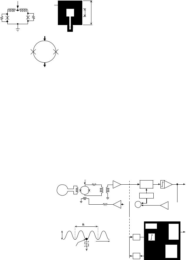
The rf SQUID was popular in the early days of superconducting magnetometry because they required only one Josephson junction. However, in majority of low Tc commercial applications, the rf SQUIDs have been displaced by dc SQUIDs due to their greater sensitivity, although in recent years, interest in rf SQUIDs has been renewed in connection with high Tc superconductivity. The operation of SQUIDs is illustrated in Fig. 1a. The dc SQUID can be modeled as a superconducting ring interrupted by two resistively shunted Josephson junctions as in Fig. 1a (11). The Josephson junctions are superconducting quantum mechanical devices that allow passage of currents with zero voltage, and when voltage is applied to them, they exhibit oscillations with a frequency to voltage constant of 484 MHz mV. The resistive shunting causes the Josephson junctions to work in a nonhysteretic mode, which is necessary for low noise operation (9). An example of a thin-film dc SQUID, consisting of a square washer and Josephson junctions near the outside edge is shown in Fig. 1b (12,13). The usual symbol used to represent a dc SQUID is shown in Fig. 1c.
The SQUID ring (or washer) must be coupled to the external world and to the electronics that operates it (see Fig. 2a). When the dc SQUID is current biased, its I–V characteristics is similar to that of a nonhysteretic Josephson junction and the critical current I0 is modulated
232 BIOMAGNETISM
L/2 |
I |
L/2 |
SQUID |
|
|
|
|
washer |
|
|
|
||
R |
|
R |
|
|
d |
D |
JJ |
F |
JJ |
|
|
|
|
(a) |
|
|
(b) |
JJ |
JJ |
|
|
|
|
|
|
(c)
Figure 1. Thin-film dc SQUID. (a) Schematic diagram indicating inductances of the SQUID ring and shunting resistors to produce nonhysteretic Josephson junctions. (b) Diagram of a simple SQUID washer with Josephson junctions near the outer edge. (c) Symbolic representation of a dc SQUID, where the Josephson junctions are indicated by ‘x’. (Reproduced with permission from Ref. 10).
by magnetic flux externally applied to the SQUID ring. The modulation amplitude is roughly equal to F0/L (9), where F0 is the flux quantum with magnitude 2.07 10 15 Wb and L is inductance of the SQUID ring. The critical current is maximum for applied flux F ¼ nF0 and minimum for F ¼ (n þ 1/2)F0. For monotonically increasing flux the average SQUID voltage oscillates as in Fig. 2d with period equal to 1 F0. The SQUID transfer function is periodic (Fig. 2d) and to linearize it, the SQUID is operated in a feedback loop as a null detector of magnetic flux (14). Most SQUID applications use analogue feedback loop whereby a modulating flux with 1/4 F0 amplitude is applied to the SQUID sensor through the feedback circuitry (Fig. 2a,b).
The modulation, feedback signal, and the flux transformer output are superposed in the SQUID, amplified, and demodulated in a lock-in detector fashion. The demodulated output is integrated, amplified, and fed back as a flux to the SQUID sensor to maintain its total input close to zero. The modulation flux superposed on the dc SQUID transfer function is shown in Fig. 2d and the modulation frequencies are typically several hundreds of kilohertz.
For satisfactory MEG operation, the SQUID system must exhibit large dynamic range, excellent interchannel matching, good linearity, and satisfactory slew rates. The analogue feedback loop is not always adequate and the dynamic range can be extended by implementing digital integrator as shown in Fig. 2c, and by utilizing the flux periodicity of the SQUID transfer function (15). The dynamic range extension works in the following manner: The loop is locked at a certain point on the SQUID transfer function and remains locked for the applied flux in the range of 1 F0, Fig. 2d. When this range is exceeded, the loop lock is released and the locking point is shifted by 1 F0 along the transfer function. The flux transitions along the transfer function are counted and are merged with the signal from the digital integrator to yield 32 bit dynamic range. This ‘‘flux slipping’’ concept can also be implemented using four-phase modulation (16), where the feedback loop jumps by F0/2 and can also provide compensation for the variation of SQUID inductance with the flux changes.
Flux Transformers
The purpose of flux transformers is to couple the SQUID sensors to the measured signals and to increase the overall magnetic field sensitivity. The flux transformers are superconducting and consist of one or more pickup coil(s) that are exposed to the measured fields. The pickup coil(s) are connected by twisted leads to a coupling coil that inductively couples the measured flux to the SQUID ring (as
Figure 2. Examples of SQUID electronics, where the SQUID is operated as a null detector. (a) SQUID sensor is coupled to an amplifier. (b) Analogue feedback loop. (c) Digital feedback loop using digital signal processor (DSP) or a programmable logic array (PGA). (d) Feedback loop modulation. (Adapted with permission from Ref. 10).
|
SQUID front end |
|
|
|
|
|
Analog feedback loop |
|
|
Flux |
Bias current |
Amplifier |
Integrator |
|
transformer |
Lock-in |
|
Analog |
|
|
|
detector |
|
output |
|
SQUID |
|
|
|
Pickup |
|
Oscillator |
|
|
|
|
|
|
|
coil |
|
Σ |
AR |
(b) |
|
Feedback |
|||
|
|
|
||
|
(a) |
|
|
|
|
|
Digital feedback loop |
|
|
|
1Φ o |
Counter |
|
|
|
|
|
|
|
|
|
|
Merge |
Digital |
|
|
|
output |
|
∆V |
|
|
|
|
|
A/D |
|
|
|
|
|
|
|
|
|
|
Applied |
DSP |
|
|
Lock |
flux, Φ |
|
|
|
point |
|
and/or |
|
(d) |
Time |
D/A |
PGA |
(c) |
|
|
|
|
|
(a)
(c)
(b) (d) (e) (f) (g) (h) 
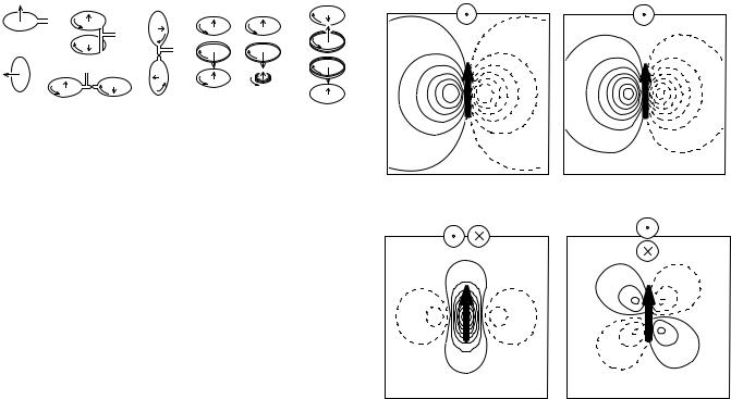
Figure 3. Examples of hardware flux transformers for biomagnetic applications. It is assumed that the scalp surface is at the bottom of the figure, (a) Radial magnetometer; (b) tangential magnetometer; (c) radial first-order gradiometer; (d) planar firstorder gradiometer; (e) radial gradiometer for tangential fields;
(f) second-order symmetric gradiometer; (g) second-order asymmetric gradiometer; (h) third-order gradiometer. (Reproduced with permission from Ref. 10).
shown in Fig. 2a). Because the flux transformers are superconducting, their gain is noiseless and their response is independent of frequency. The flux transformer pickup coil can have diverse configurations as shown in Fig. 3. A single loop of wire acts as a magnetometer and is sensitive to the magnetic field component perpendicular to its area, Fig. 3a and b. Two magnetometer loops can be combined with opposite orientation and connected by the same wire to the SQUID sensor. The loops are separated by a distance b and such a device is called a first-order gradiometer Fig. 3c–e, and the distance b is referred to as gradiometer baseline. The magnetic fields detected at the two coils are subtracted and the gradiometer acts as a spatial differential detector (this differential action is comparable to differential detection of electric signals (e.g., in electroencephalography, EEG). Fields induced by distant sources will be almost completely canceled by a gradiometer because both its coils will detect similar signals. On the other hand, near sources will produce markedly different fields at the two gradiometer coils and will be detected. Thus the gradiometers diminish the effect of the environmental noise that is typically generated by distant sources while remaining sensitive to near sources (e.g., neural sources). Similarly, first-order gradiometers can be combined with opposing polarity to form second-order gradiometers (Fig. 3f,g) and second-order gradiometers can be combined to form third-order gradiometers, (Fig. 3h). The flux transformers in Fig. 3 are called hardware flux transformers, because they are directly constructed in hardware by interconnecting various coils.
The main types of flux transformers used in commercial practice as the primary sensors are magnetometers (Fig. 3a), radial gradiometers (Fig. 3c), and planar gradiometers (Fig. 3d). These different sensor types will measure different spatial pattern of magnetic flux when placed over a current dipole as shown in Fig. 4. The radial magnetometer produces a field map with one maximum and one minimum, symmetrically located over the dipole with zero field measured directly above the dipole (Fig. 4a). The radial gradiometer in Fig. 4b produces similar field pattern as the magnetometer, except that the pattern is spatially tighter since it subtracts two field patterns measured at different distances from the dipole. The planar gradiometer field patterns are quite different from that of the
BIOMAGNETISM 233
(a) Magnetometers |
(b) Radial grads. |
(c) Planar grads. |
(d) Planar grads. |
Figure 4. Response to a point dipole of several flux transformer types. A tangential dipole is positioned 2 cm deep in a semi infinite conducting space bounded by x3 ¼ 0 plane and its field is scanned by a flux transformer with its sensing coil positioned at x3 ¼ 0. Dipole position is indicated by a black arrow. Dimensions of each map are 14 14 cm. Schematic top view of the flux transformers is shown in the upper part of each figure. Solid and dashed lines indicate different field polarities. (a) Radial magnetometer; (b) radial gradiometer with 4 cm baseline; (c) planar gradiometer with 1.5 cm baseline aligned for maximum response; (d) planar gradiometer with 1.5 cm baseline aligned for minimum response. (Reproduced with permission from Ref. 10).
radial devices. If the two coils of the planar gradiometer are aligned perpendicular to the dipole, as in Fig. 4c, the planar gradiometer exhibits a peak directly above the dipole; if the two coils were aligned parallel to the dipole, the planar gradiometer exhibits a weak, clover-leaf pattern. When two orthogonal planar gradiometers are positioned at the same location, their two independent components can determine orientation of the current dipole located directly under the gradiometers (17).
In the absence of noise, there are no practical differences between these types of flux transformers. However, in the presence of noise, the signal-to-noise ratios (SNR) can differ greatly, resulting in significant performance differences between devices. For MEG applications, the magnitude of both the detected brain signal and environmental noise increases with increasing gradiometer baseline (distance between coils). Since the signal and noise functional dependencies on baseline are different, SNR exhibits a peak corresponding to an optimum baseline of 3–8 cm for first-order radial gradiometers (10). Magnetometers can be thought of as gradiometers with very long baseline
234 BIOMAGNETISM
and are not optimal because they can be overly sensitive to environmental noise. Planar gradiometers have good SNR for shallow brain sources but are suboptimal for deeper sources due to their short baselines resulting in poor depth sensitivity. Too long a baseline can also result in greater sensitivity to noise sources arising from the body itself, such as the magnetic field of the heart that may then contaminate the MEG signal. A detailed comparison of gradiometer design and performance can be found in (10).
Noise Cancelation
Introduction. Since biomagnetic measurements must be made in real world settings, the influence of noise on the measurements is a major concern in the design of biomagnetic instrumentation. Environmental noise affects biomagnetometer systems even when they are operated within shielded rooms. Environmental noise results from moving magnetic objects and currents (cars, trains, elevators, power lines, etc.). These noise sources are many orders of magnitude larger than signals of biomagnetic origin as shown in Fig. 5a. Note also, that only SQUID magnetometers have sufficient sensitivity for measuring biomagnetic signals of interest [atomic magnetometers are not yet suitable for biomagnetic applications (19)]. For MEG applications, the resolution or white noise level of the sensors should be much less than the ‘‘noise’’ level of brain activity ( 30 fT Hz1/2). An example of background brain activity is shown in Fig. 5b. Also, certain MEG signal
interpretation methods require the white noise to be as low as possible, however, the noise level cannot be made lower than the contribution of noise from the cryogenic vessel (dewar) itself. As a compromise, the majority of the
existing MEG systems exhibit intrinsic noise levels of <10 fT Hz1/2 (typically 5 fT Hz1/2), yet are able to tol-
erate unwanted environmental noise many orders of magnitude greater.
Magnetic Shielding. Magnetic shielding is the most straightforward, though most costly method for reduction of environmental noise. A variety of shielded rooms have been used for biomagnetic applications and their relative shielding performance is shown in Fig. 6. The simplest shielding is accomplished through eddy currents by using a thick layer of high conductivity metal (20). Eddy current shielding is not effective at low frequencies, and therefore shielded rooms utilize high permeability m-metal, which depending on the number of layers, can provide attenuation in the range from 30 to 105 (21–24). Low frequency attenuation of nearly 108 was demonstrated with a wholebody, high Tc superconducting shield (25).
Environmental noise can also be reduced by active shielding, which can be employed either in unshielded environments (26), or in combination with shielded rooms (24,27,28). Active shielding system consists of a reference magnetometer, feedback electronics, and a set of compensating coils. The references measure the environmental noise and provide a signal that is amplified and fed into the
Figure 5. Environmental and brain generated noise. (a) Comparison of biomagnetic fields, environmental noise, and sensitivity in 1 Hz bandwidth of various types of magnetometers. (b) Spontaneous brain activity and the system noise measured in an unshielded environment, noise cancelation by synthetic third-order gradiometer, primary sensors are radial first-order gradiometers with 5 cm baseline. Control trace was collected with no subject in the helmet, large lines correspond to signals due to nearby rotating machinery. Eyes closed and open were collected with the subject in the MEG helmet. The presence of alpha activity (peak at 8 Hz) is visible in the eyes closed condition. (Reproduced with permission from Ref. 18).
Combination of synthetic
methods and standard
µ-metal shields
Shielded rooms for
biomagnetic applications
|
8 |
|
|
(f) Whole body |
sup |
|
|
|
|
|
|
|
|
|||||||
|
10 |
|
|
|
|
|
|
|
|
|
|
|
|
|
|
|
|
|||
|
|
|
|
|
|
|
|
|
|
|
|
er |
|
|
|
|
|
|
|
|
|
|
|
|
|
|
|
|
|
|
|
|
|
c |
|
|
|
|
|
|
|
|
|
|
|
|
|
|
|
|
|
|
|
|
o |
|
|
|
|
|
|
|
|
|
|
|
|
|
|
|
|
|
|
|
|
|
n |
|
|
|
|
|
|
|
|
|
|
|
|
|
|
|
|
|
|
|
|
d |
|
|
|
|
|
|
|
|
|
|
|
|
active |
|
|
|
|
|
|
|
u |
|
|
|
|
||
|
107 |
(e) Berlin room |
|
|
|
|
|
|
|
|
ct |
|
|
|
||||||
|
|
|
|
|
|
|
|
|
|
|
|
ing s |
|
|
||||||
|
|
|
|
|
|
|
|
|
|
|
|
|
|
|
|
|
|
hi |
|
|
|
|
|
|
|
|
|
|
|
|
|
|
|
|
|
|
|
|
e |
|
|
|
|
|
|
|
|
|
room |
|
|
|
|
|
|
|
|
|
|
ld |
|
|
|
106 |
|
|
|
|
|
|
|
|
|
-met |
|
|
|
|
|||||
|
|
Berlin |
|
|
|
|
|
|
|
|
|
|||||||||
|
|
(d) |
|
|
|
|
|
|
|
|
n |
µ |
|
|
al |
s |
|
|
||
|
|
|
|
|
|
|
|
|
|
|
|
|
|
|
||||||
factor |
|
|
|
|
|
|
|
|
|
tio |
|
|
|
|
|
hield |
|
|
||
|
|
|
|
|
|
|
|
|
a |
|
|
|
|
|
|
|
|
|
||
5 |
|
|
|
|
|
|
|
enu |
|
|
|
|
|
|
|
|
|
|
||
|
|
|
|
|
|
tt |
|
|
|
|
|
|
|
|
|
|
|
|||
10 |
|
|
|
|
|
a |
|
|
|
|
|
|
|
|
|
|
|
|
||
|
|
|
|
|
gh |
|
|
|
|
|
|
|
|
|
|
|
|
|
||
|
|
|
(c) |
Hi |
|
|
|
|
|
|
|
|
|
|
|
|
|
|||
Attenuation |
|
|
|
|
|
|
|
|
|
|
|
|
|
|
|
|
|
|||
104 |
|
|
|
|
|
|
|
|
|
|
|
|
|
|
|
|
|
|
|
|
103 |
|
|
|
|
|
|
|
-metal |
shields |
|
|
|
|
|
||||||
|
|
|
|
|
|
|
µ |
|
|
|
|
|
|
|
|
|
|
|
||
|
100 |
(b) |
Standard |
|
|
|
|
|
|
|
|
|
shields |
|||||||
|
|
|
|
|
|
|
|
|
|
|
|
|
|
|
||||||
|
|
|
|
|
|
|
|
|
|
|
|
|
|
|
|
|
|
|||
|
10 |
|
|
|
|
|
|
|
|
|
|
Eddy |
current |
|
|
|||||
|
|
|
|
|
|
|
|
|
|
|
|
|
|
|
|
|
||||
|
|
|
|
|
|
|
|
|
|
(a) |
|
|
|
|
|
|
||||
|
1 |
|
|
|
|
|
|
|
|
|
|
|
|
|
|
|
|
|
||
|
0.11 |
|
|
|
|
1 |
|
|
|
|
|
10 |
|
|
|
100 |
||||
|
0.01 |
|
|
|
|
|
|
|
|
|
|
|
|
|||||||
Frequency (Hz)
BIOMAGNETISM 235
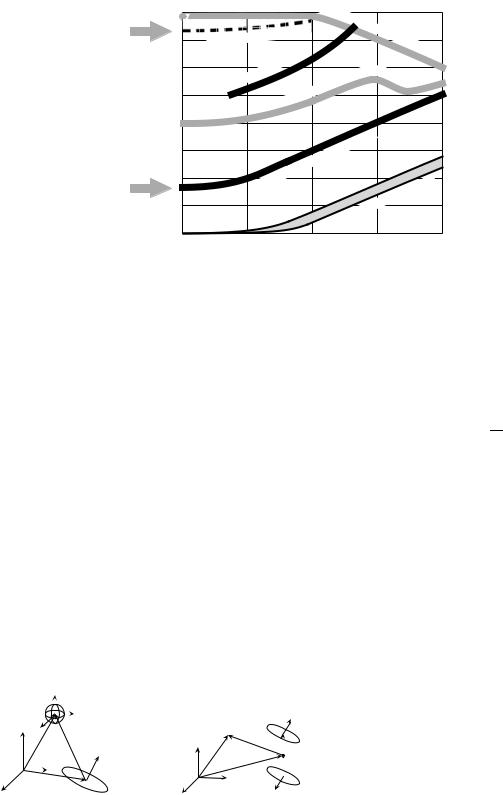
Figure 6. Noise attenuation of various shielded rooms as a function of frequency.
(a) Eddy current Al rooms. (b) Standard m- metal rooms used for MEG applications. (c,d) High attenuation m-metal rooms. (e) Combination of high attenuation m-metal room in ‘‘d’’ and active shielding. (f) Wholebody high temperature superconducting shield. (Adapted with permission from Ref. 18).
compensating coils to reduce the noise. In general, the active shielding reduces the magnetic field noise due to far field sources and is effective only for magnetometers with no noise cancelation, while it has only a small effect on first-order gradiometers or magnetometers with noise cancelation. For higher order gradiometers, active shielding actually degrades system performance since the active coils can produce higher order gradients that are larger than that of the environmental noise.
Noise Reduction Using Higher Order Gradients. Since hardware noise cancelation (shielding or active noise cancelation) is usually not sufficient, additional methods, implemented in software or firmware, are employed. These methods either incorporate information from additional reference sensors or operate directly on the primary sensors. The reference sensors are typically a combination of SQUID magnetometers and gradiometers and the noise is canceled by synthesizing either higher order gradiometers or adaptively minimizing noise. The principle of synthetic gradiometer operation is similar for all gradiometer orders, and the method is illustrated for first-order gradiometer synthesis in Fig. 7a (29). The primary magnetometer
|
|
|
|
|
Three component |
1st gradient |
Primary |
|||||||
|
r3 |
|
reference magnetometer |
tensor |
1st-order |
|||||||||
|
|
|
|
|
r2 |
|
reference |
gradiometer |
||||||
x3 |
r1 |
|
|
|
gradiometer |
|
p |
|||||||
|
|
|
|
|||||||||||
|
|
|
|
|
|
|
|
b2 |
||||||
u2 |
|
b |
|
|
|
|
|
|
|
|||||
|
|
|
|
|
|
|
|
|||||||
|
|
p |
x3 u ′ |
|
Center |
|||||||||
|
x2 |
|
|
|
||||||||||
|
|
|
|
|
|
|
|
|
|
b1 |
||||
|
|
|
|
|
|
|
|
|
u |
|
||||
|
|
u1 |
|
|
|
|
|
|
|
|
|
|
||
x1 |
|
|
|
|
|
x2 |
−p |
|||||||
|
Primary |
(a) |
|
|||||||||||
|
x1 |
|
(b) |
|||||||||||
magnetometer
Figure 7. An illustration of gradiometer synthesis. (a) Synthesis of a first-order gradiometer from a primary magnetometer sensor and a vector magnetometer reference. (b) Synthesis of a secondorder gradiometer from hardware first-order gradiometer and a first-gradient tensor reference. (Adapted from Ref. 30).
detects the magnetic field component parallel to its coil normal, p (unit vector). The three reference magnetometers are orthogonal and their vector output, r, corresponds to the environmental field at the reference location, r B. Then, if ap is the primary magnetometer gain and ar the reference gain (identical for all three references), the synthetic first-order gradiometer, g(1), can be derived as
ap |
|
|
gð1Þ ¼ mp ar |
ðp rÞ app G b |
ð1Þ |
where b is the gradiometer baseline (a vector connecting the primary sensor and the reference centers), and G is the first gradient tensor at the coordinate origin. Equation 1 states that the synthetic first-order gradiometer is a projection of the first-gradient tensor to the primary magnetometer orientation, p, and the baseline, b. To synthesize a second-order gradiometer, a primary hardware or synthetic first-order gradiometer, and a tensor first-gradient reference are used (Fig. 7b). Similar to Eq. 1, it can be shown that the synthetic second-order gradiometer output is a projection of the second gradient tensor to the coil orientation p and the firstand second-order gradiometer baselines b1 and b2. Synthesis of thirdand higher order gradiometers is similar (29).
Adaptive methods can also be applied in addition to the synthetic gradiometers and can incorporate the same references as the gradiometers, but their coefficients are explicitly computed to minimize correlated noise (29). The advantage of synthesizing higher order gradiometers is that their coefficients are universal, independent of the noise character or sensor orientation (18). In contrast, the coefficients determined to adaptively minimize background noise are not universal because they depend on the noise character and sensor orientations (18) and assume that the noise environment is unchanging.
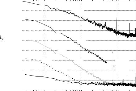
The noise cancelation achieved by various methods is illustrated in Fig. 8. The upper trace (a) shows the magnetic field noise outside a shielded room; and trace (b) shows the field noise after attenuation by the shielded room. The difference of the two slopes is due to the
236 BIOMAGNETISM
Figure 8. Reduction of environmental noise by a moderately shielded room, synthetic gradiometers, and adaptive methods. (a) Magnetic field noise outside a shielded room. (b) Field noise after attenuation by the shielded room. (c) Noise reduction by hardware first-order gradiometer with 5 cm baseline. (d) Noise reduction by synthetic third-order gradiometer (nearly four orders of magnitude lower noise than that of a shielded magnetometer in ‘‘b’’). (e) Noise reduction by addition of adaptive methods to synthetic third-order gradiometer. (Adapted from Ref. 31).
|
1 µT |
|
|
|
|
|
|
|
|
|
|
|
|
|
|
|
|
|
(a) |
|
|
|
|
|
|
Unshielded |
|
|
|
|
|
||
|
100 nT |
|
|
|
|
|
|
|
mags |
|
|
|
|
|||
|
|
|
|
|
|
|
|
|
|
|
|
|
||||
|
|
|
|
|
|
|
|
|
|
|
|
|
|
|
|
|
|
10 nT |
(b) |
|
|
|
|
|
|
|
|
|
|
|
|
|
|
|
|
|
|
|
|
|
|
|
|
|
|
|
|
|
|
|
|
1 nT |
|
|
|
|
|
|
|
|
Magnetometers |
|
|
|
|
||
Hz) |
|
(c) |
|
|
|
|
|
|
|
|
|
|
|
|||
100 pT |
|
|
|
|
|
|
|
|
|
|
|
|
||||
(rms/ |
|
|
|
|
Hardware |
|
|
|
|
|
|
|||||
|
|
|
|
|
|
|
|
|
|
|
||||||
Noise |
10 pT |
|
|
|
|
1st |
|
|
|
|
|
|
|
|
||
|
|
|
|
|
|
|
|
|
|
|
|
|
|
|||
|
|
|
|
|
|
|
|
|
|
|
|
|
|
|
||
|
(d) |
|
|
|
|
|
- |
|
|
|
|
|
|
|
||
|
Synthetic |
|
|
|
|
order |
gradiometers |
|
|
|
|
|||||
|
|
|
|
|
|
|
|
|
|
|
||||||
|
1 pT |
|
3rd- |
|
|
|
|
|
|
AK3b |
|
|||||
|
|
|
|
|
|
|
|
|
|
|
||||||
|
|
|
|
|
|
|
|
|
|
|
|
|||||
|
100 fT |
|
|
|
|
order |
grads |
|
|
|
shielded |
|||||
|
(e) |
|
|
|
|
|
|
|
|
|
room |
|
||||
|
10 fT |
Synth. |
|
|
|
|
|
|
|
|
|
|
|
|
|
|
|
3rd-order grads. |
|
|
|
|
|
|
|
|
|
|
|
||||
|
|
|
|
|
|
|
|
|
|
|
|
|
||||
|
1 fT |
and adaptive noise cancel. |
|
|
|
|
|
|
|
|
||||||
|
|
0.05 |
0.1 |
0.2 |
|
|
|
0.5 |
1 |
2 |
5 |
10 |
20 |
|||
|
|
|
|
|
|
|||||||||||
Frequency (Hz)
frequency dependent eddy current shield that is part of the room. Hardware first-order radial gradiometers with 5 cm baseline reduce noise by nearly a factor of 100; and (c) a synthetic third-order gradiometer; (d) reduces the noise by almost another factor of 100. The low frequency environmental noise can further be reduced by adaptive method
(e). The combination of all methods in Fig. 8 achieves attenuation of >107 at low frequencies.
Additional noise reduction methods can be employed in systems with a large number of channels. The simplest method is spatial filtering using Signal Space Projection (SSP) (32–34), which projects out from the measurement the noise components oriented along specific spatial vectors in signal space. The method works best when the signal and noise subspaces are nearly orthogonal. Related to SSP is noise elimination by rotation in signal space (35), which avoids loss of degrees of freedom encountered in SSP. These methods are discussed further in the Signal Interpretation section. More recently Signal Space Separation (SSS) has been proposed as a noise cancelation method in MEG (36). This approach was first proposed by Ioannides et al. (37) and reduces environmental noise by retaining only the ‘‘internal’’ component of the spherical expansion of the measured signal. This method can be applied to a number of problems inherent in biomagnetic measurements, including environmental noise reduction and motion compensation.
Cryogenics
The sensing elements of a biomagnetometer system (SQUIDs, flux transformers, and their interconnections) are superconducting and must be maintained at low temperatures. Since all commercial systems use low temperature superconductors, they must be operated at liquid He temperatures of 4.2 K. These temperatures can be achieved
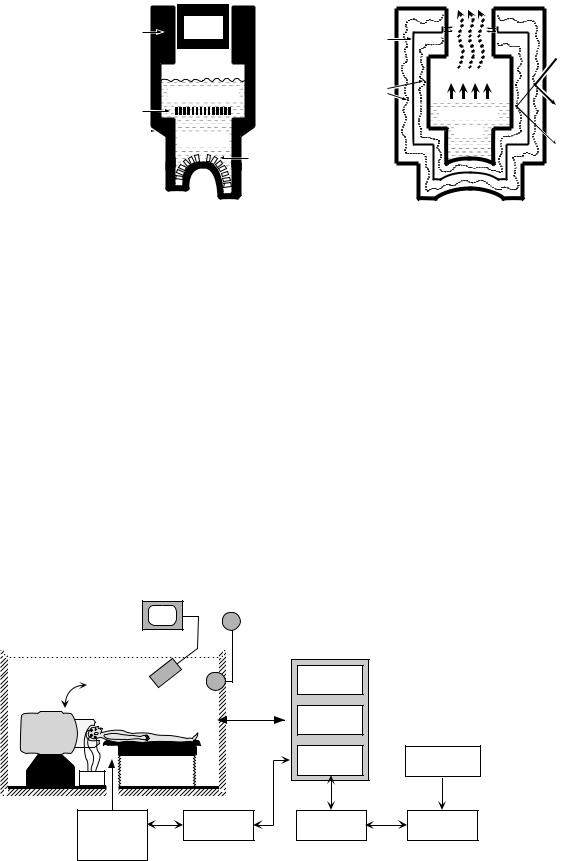
either with cryocoolers or by a cryogenic bath in contact with the superconducting components. The cryocoolers are attractive because they eliminate the need for periodic refilling of the cryogenic container. However, because they contribute magnetic and electric interference, vibrational noise, thermal fluctuations, and Johnson noise from metallic parts (38), they are not yet commonly used in MEG instrumentation. Present commercial biomagnetometer systems rely on cooling by liquid He bath in a nonmagnetic vessel with an outer vacuum space also referred to as a Dewar. An example of how the components may be organized within the Dewar for an MEG system is shown in Fig. 9a (39). The primary sensing flux transformers are positioned in the Dewar helmet area. The reference system for the noise cancelation is positioned close to the primary sensors and the SQUIDs with their shields are located at some distance from the references, all immersed in liquid He or cold He gas. The Dewar is a complex dynamic device that incorporates various forms of thermal insulation, heat conduction, and radiation shielding, as shown Fig. 9b. Most commercial MEG and MCG systems have reservoirs holding up to 100 L of liquid He and can be operated for periods of several days before refilling. An excellent review of the issues associated with the Dewar construction is presented in (38).
Biomagnetometer Systems: Overview
Even though magnetic fields have been detected from many organs, so far the most important application of biomagnetism has been the detection of neuromagnetic activity of the human brain. This interest led to the development of sophisticated commercial MEG systems. The current generation of these systems consists of helmet shaped multisensor arrays capable of measuring activity
|
|
|
BIOMAGNETISM |
237 |
|
|
Escaping vapors |
|
|
|
|
(warm, ~ room T) |
|
|
Vacuum |
Vacuum |
Vapor |
|
|
space |
plug |
cooled |
|
|
|
|
heat |
Incoming |
|
|
|
shields |
heat |
|
|
|
Cold vapors |
radiation |
|
|
|
|
|
|
|
Liquid helium |
Super- |
|
|
|
insulation |
|
|
|
SQUIDs |
|
Heat |
|
|
|
Liquid He4 |
|
||
|
reflected |
|
||
|
|
|
||
Calibration |
|
|
|
|
|
4.2K |
by super- |
|
|
points (for head |
References |
|
insulation |
|
localization) |
|
Sensing coils |
|
|
|
|
|
|
(a) (b)
Figure 9. Schematic diagram of cryogenic containers used for whole-cortex MEG. (a) Placement of various MEG components relative to the cryogenic Dewar. (b) Principles of the Dewar operation. Reproduced with permission from (10).
simultaneously from the entire cerebrum. In contrast, multichannel magnetocardiogram (MCG) systems consist of a flat array of radial or vector devices (40–45) or systems with a smaller number of channels operating at liquid N2 temperatures (46–51) for better placement over the chest directly above the heart. These flat array systems can also be placed over other areas of the body to measure peripheral nerve, gastrointestinal, or muscle activity. These systems can even be placed over the maternal abdomen to measure heart and brain activity of the fetus and a custom shaped multichannel array specifically designed for fetal measurements has recently been introduced (39,52).
MEG Systems. A diagram of a generic MEG system is shown in Fig. 10. The SQUID sensors and their associated flux transformers are mounted within a liquid He dewar suspended in a movable gantry to allow for supine or seated patient position. The patient rests on an adjustable chair or
a bed. All signals are preamplified and transmitted from the shielded room to a central workstation for real-time acquisition and monitoring of the magnetic signals. At present, the majority of MEG installations use magnetically shielded rooms, however, progress is being made toward unshielded operation (18,40). The MEG measurements are often complemented by simultaneous EEG measurements or peripheral measures of muscle activity or eye movement. Most MEG installations have provisions for stimulus delivery in order to study brain responses to sensory stimulation and video and intercom systems in order to interact with the patient from outside the shielded room. Multichannel MEG systems are commercially available from a number of manufacturers (39,53–56).
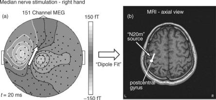
For MEG localization of brain activity to be useful, particularly in clinical applications, it must be accurately known relative to brain anatomy. The anatomical information is usually obtained by magnetic resonance imaging
Magnetically |
|
Video |
Intercom |
|
|
shielded room |
|
monitor |
|
System |
|
(optional) |
|
|
|
|
|
|
|
|
|
electronics |
|
Adjustable dewar |
Video |
|
EEG |
|
|
and gantry |
|
camera |
|
electronics |
|
|
|
|
|
SQUID |
|
|
|
|
|
electronics |
|
|
|
|
|
DSP |
Data |
|
|
|
|
processing |
interpretation |
|
EEG |
|
|
|
|
Stimulus |
Auditory |
Stimulus |
Acquisition |
Analysis |
|
|
Visual |
computer |
work station |
work stations |
|
interface |
Somatosens. |
|
|
|
|
|
|
Other |
|
|
|
Figure 10. Schematic diagram of a typical MEG installation in a magnetically shielded room. (Reproduced with permission from Ref. 10).
238 BIOMAGNETISM
(MRI), and the MRI images are required during the MEG interpretation phase. The registration of the MEG sensors to the brain anatomy is performed in two steps. First, the head position relative to the MEG sensor array is determined in order to accurately position MEG sources within a head-based coordinate system. Second, the head position relative to the MRI anatomical image is determined to allow transfer of MEG sources to the anatomical images. There are different methods for such registration. The simplest one uses a small number of anatomical markers positioned on identical locations on the head surface that can be measured both by MEG and MRI (e.g., small coils for MEG and lipid contrast markers for MRI) usually placed at anatomical landmarks near the noise and ears (18). To improve localization accuracy, the head shape can be digitized in the MEG coordinate system by a device mounted on the dewar (57) or by the MEG sensors (10). The surface of the head can also be constructed from segmented MRI and the transformation between the two systems can be determined by alignment of the two surfaces (58–60).
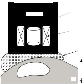
Biosusceptometers. A somewhat different system design is encountered in biomagnetometer systems used for the measurement of magnetic materials in the human body, such as iron content in the liver or magnetic contaminants in the lung. These instruments contain both SQUID sensing coils and a superconducting magnet operated in persistent mode. The system is suspended over the patient’s body on a bed with a waterbag placed between the patient and dewar to provide continuity of the diamagnetic properties of body tissue. Figure 11 illustrates the layout of a biosusceptometer system for liver measurements with a patient in a supine position on a moveable bed. The patient
|
(a) SQUID |
gradiometer |
|
Liquid He |
|
Superconducting |
|
(b) |
magnet |
|
(c) Water bag |
Liver |
|
|
(d) |
Figure 11. Schematic diagram of a liver susceptometer. (a) SQUID gradiometer. (b) Superconducting magnet. (c) Bag filled with water to simulate the diamagnetism of human body tissue. (d) Patient on a bed that is vertically movable. (Reproduced with permission from Ref. 61).
is moved vertically relative to the SQUID gradiometermagnet system and flux changes due to the susceptibility of the liver are monitored. These measures of magnetic moment can then be used to estimate the concentration of the paramagnetic compounds within the liver (62–64).
Signal Interpretation
Biomagnetometers measure the distribution of magnetic field outside of the body. Although the observed field patterns provide some information about the underlying physiological activity, ideally one would like to invert the magnetic field and provide a detailed image of the current distribution within the body. Such inversion problems are nonunique and ill defined. The nonuniqueness is either physical (65) or mathematical due to being highly underdetermined (i.e., there are many more sources than sensors). In order to determine the current distribution, it is necessary to provide additional information, constraints, or simplified mathematical models of the sources. The field of source modeling in both MEG and MCG has been an intensive area of study over the last 20 years. In the following section we shall review briefly various methods of source analysis as it is applied to MEG, although these methods apply to other biomagnetic measurements such as MCG, with the main difference being the physical geometry of the conductor volumes containing the sources. For detailed reviews of mathematical approaches used in biomagnetism (see 66–69).
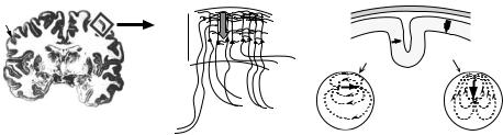
Neural Origin of Neuromagnetic Fields. Magnetic fields of the brain measured by MEG are thought to be the primarily due to activation of neurons in the gray matter of the neocortex, whereas action potentials in the underlying fiber tracts (white matter) have been shown to produce only poorly synchronized quadrupolar sources associated with weak fields (70,71). Some subcortical structures have also been shown to produce weak yet measurable magnetic fields, but are difficult to detect without extensive signal processing (72,73). The generation of magnetic fields in the human brain is illustrated in Fig. 12. The neocortex of the brain (shown in Fig. 12a) contains a large number of pyramidal cells arranged in parallel (Fig. 12b) that in their resting state maintain an intracellular potential of ca. 70 mV. Excitatory (or inhibitory) synaptic input near the cell body or at the superficial apical dendrites results in the flow of charged ions across the cell membrane producing a graded depolarization (or hyperpolarization) of the cell. This change in polarization results in current flow inside the cell, called impressed current and corresponding return or volume currents that flow through the extracellular space in the opposite direction. Studies carried out in the early 1960s (74,75) demonstrated that these extracellular or volume currents are main generators of electrical activity measured in the electroencephalogram or EEG. The combination of excitatory and inhibitory synaptic inputs to different cortical layers can produce a variety of sink and source patterns through the depth of the cortex, each associated with current flow along the axes of elongated pyramidal cells toward or away from the cortical surface.
Cortex |
|
|
Skull |
|
|
|
Dendrites |
Cortex |
CSF |
||
Cortex |
|
|
|||
|
cell bodies Tangential |
Radial |
|||
(2-5 mm) |
|
|
dipole |
dipole |
|
|
|
Axons |
|
|
|
|
|
(output) |
|
(c) |
|
|
|
|
|
||
Coronal section |
Synaptic input |
|
|
||
|
|
|
|||
(a) |
(b) |
Produces external |
No external |
||
magnetic field |
magnetic field |
||||
|
|
||||
|
|
|
(d) |
(e) |
|
BIOMAGNETISM 239
Figure 12. Origin of the MEG signal. (a) Coronal section of the human brain. The neocortex is indicated by dark outer surface. (b) Pyramidal cells in the cortex have vertically oriented receptive areas (dendrites). Depolarization of the dendrites at the cortical surface due to excitatory synaptic input results in Naþ ions entering the cell producing a local current source and a current sink at the cell body, resulting in intracellular current flowing toward the cell body (arrow). (c) The cortex has numerous sulci and gyri resulting in currents flowing either tangentially or radially relative to the head surface. (d) Tangential currents will produce magnetic fields that are observable outside the head if modeled as a sphere. (e) Radial currents will not produce magnetic fields outside of the head if modeled as a sphere. (Adapted from Ref. 10).
Synchronous activity in large populations of these cells summate to produce the positive and negative time-vary- ing voltages measured at the scalp surface in the EEG (76).
Okada et al. (77) carried out extensive studies over the last 20 years on the neural origin of evoked magnetic fields using small array ‘‘microSQUID’’ systems to measure directly magnetic fields from in vitro preparations in the turtle cerebellum and mammalian hippocampus. These studies have shown that although both extracellular and intracellular currents may contribute to externally measured magnetic fields, it is primarily intracellular or impressed currents flowing along the longitudinal axis of pyramidal cells that are the generators of evoked magnetic fields. A recent review of this work is presented in (78). Note that, since MEG measures mainly intracellular currents and EEG the return volume currents, the pattern of electrical potential over the scalp due to an underlying current source will reflect current flow in opposite direction to that of the magnetic field, as has been demonstrated in physical models (79) and human brain activity (80). In addition, activation of various regions of the enfolded cortical surface (the gyri and sulci) will result in current flow that is either radial or tangential to the scalp surface, respectively (Fig. 12c). If the brain is modeled as a spherical conducting volume, then due to axial symmetry it can be shown that only the tangential currents will produce fields outside the sphere (81) (Fig. 12d and e). Using in vivo preparations in the porcine brain, it has been experimentally demonstrated that, in contrast to the EEG, magnetic fields are relatively undistorted by the presence of the skull, and are generated primarily in tangentially oriented tissue (78). It has been recently shown, however, that MEG is insensitive only to a relatively small percentage of the total cortical surface in humans due to this tangential constraint (82). There is some uncertainty as to the extent of cortical activation typically measured by MEG. Current densities in the cortex have been estimated to be on the
order of 50 pA m mm2(83) suggesting that cortical areas of at least 20 mm2 must be activated in order to produce a sufficiently large external field to be observed outside the head (66,68). However, current densities as high as 1000 pA m mm2 have been recorded in vitro (77) indicating that much smaller areas of activation may be observed magnetically.
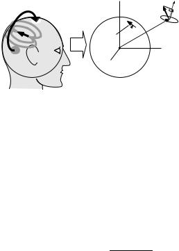
Equivalent Current Dipoles. The equivalent current dipole or ECD (81,84) is the oldest and most frequently used model for brain source activity. It is based on the assumption that activation of a specific cortical region involves populations of functionally interconnected neurons (macrocolumns) within a relatively small area. When measured from a distance, this local population activity can be modeled by a vector sum or ‘‘equivalent’’ current dipole that represents the aggregate activity of these neurons. The ECD analysis proceeds by estimating a priori the number of equivalent dipoles and their approximate locations, and then adjusting the dipole parameters (location and orientation) by a nonlinear search that minimizes differences between the field computed from the dipole model and the measured field (Fig. 13). This can be done at one time sample, or it can be extended to a time segment, where several dipoles are assumed to have fixed positions in space, but variable amplitude. Such models are referred to as ‘‘spatiotemporal’’ dipole models (85). The dipole fit procedures require the calculation of the magnetic field produced by a current dipole at each sensor: also termed the forward solution. Since the frequency range of interest for biomagnetic fields is <1 kHz, the quasistatic approximations of Maxwell’s equations apply. If the head is assumed to be approximately spherical in shape it can be represented by a uniformly conducting sphere and the radial magnetic field of an ECD with magnitude q, is given by the radial component of the well-known Biot– Savart law, Brad(r) ¼ B(r) r/jrj, where the Biot–Savart
240 |
BIOMAGNETISM |
|
|
|
|
|
|
|
z |
|
|
p |
|
|
|
|
|
B (r) |
|
|
B |
|
|
|
B coil = B (r ) |
p |
|
|
|
q |
a |
|||
|
|
|
|
|
||
|
q |
|
|
Magnetometer |
|
|
|
|
|
r |
|
||
|
|
|
|
|
|
|
|
Dipole |
|
|
r0 |
|
|
y
x
Conducting sphere
Figure 13. Magnetic fields due to an equivalent current dipole source will exit and reenter the head that can be modeled as a spherical shaped conducting medium. Calculation of the field magnitude (Bcoil) measured by a magnetometer coil due to a current dipole q at location r0 inside a sphere is given by the projection of the calculated vector field B(r) onto the direction normal to the surface area of the coil indicated by the unit vector p, such that Bcoil ¼ B(r) p. The orientation of q is assumed to be tangential to the sphere surface. For gradiometer devices, the measured output of the gradiometer can be calculated as the difference between the field magnitudes calculated separately at each of the coils.
vector field, B(r), is given by
B r |
m0 |
q ðr roÞ |
2 |
Þ |
|
4p jr roj3 |
|||||
ð Þ ¼ |
ð |
||||
where ro is the ECD position and r is the position where the field is measured. For multiple ECDs or continuously distributed sources, Eq. 2 will also include the sum over all sources or the integral over the volume of the conducting sphere.
Generally, the vector of the external magnetic field is produced by both the primary current density reflecting the impressed (intracellular) currents, and volume currents that produce ‘‘secondary sources’’ on the surface of the volume conductor. For complex shapes, the calculation of the external field also requires knowledge of the conductivity profile of the conducting volume. The assumption of spherical symmetry, however, simplifies the calculation, and the vector field B(r) due to a current dipole q in a sphere at location ro (Fig. 13b) is given by Sarvas (81) as
|
m0 |
|
|
BðrÞ ¼ |
|
fFq ro ½ðq roÞ r&rFg |
(3a) |
4pF2 |
|||
where |
|
|
|
|
F ¼ aðra þ r2 ro rÞ |
(3b) |
|
and |
|
|
|
rF ¼ ðr 1a2 þ a 1a r þ 2a þ 2rÞr |
|
||
|
|
ða þ 2r þ a 1a rÞro |
(3c) |
and a ¼ r ro, a ¼ jaj, r ¼ jrj and the permeability of free space m0 ¼ 4p 10 7 H m. The sensing coil measures the component of the vector field B(r) perpendicular to its surface area as shown in Fig. 13b. If the field is measured only in the radial direction, Eq. 3 simplifies to the radial component of the Biot–Savart law (Eq. 2), and the volume currents do not contribute any field. It can be seen from Fig. 13 that the definition of the origin of the theoretical
sphere relative to the head will influence the calculation of the external magnetic field and thus plays a significant role in the accuracy of the single sphere approach. Since the head is not perfectly spherical, improved accuracy of the forward solution can be achieved by using more realistic models of the conducting surfaces and boundary element methods for the calculation of the magnetic field (69), but these methods are more computationally demanding. A simple improvement over the single sphere model can be achieved by using a multiple-sphere model, where independent spheres are determined for each sensor by evaluating local head curvature in the sensor vicinity (86).
The ECD procedure is very sensitive to the SNR and dc offsets, and therefore works best when applied to averaged brain responses that are well time locked to a sensory or motor event and requires an accurate estimate of signal baseline (e.g., prestimulus activity). This approach has proven useful for modeling simple patterns of focal brain activity, yet is compromised by interaction or ‘‘cross-talk’’ between simultaneously active sources, requiring that the number of dipoles be correctly specified. Also, ECD models do not correctly describe spatially ‘‘extended’’ sources: areas of cortical activity that may extend over an area of several square centimeters.
Minimum Norm. The dipole model assumes that the brain activity is localized in one or several small areas of the brain. Sometimes it is required to obtain a more general solution without an a priori assumption about the source distribution. This can be obtained by minimum norm methods, first proposed for MEG by Ha¨ma¨la¨inen and Ilmoniemi (84). This inverse problem is underdetermined, solutions are diffuse, and the unweighted minimum norm favors solutions close to the sensors. The minimum norm method has subsequently been adapted to produce more localized solutions. The algorithm, FOCal Undetermined System Solution (FOCUSS) utilizes a recursive linear estimation based on weighted pseudoinverse solution (87) and the Minimum Current Estimate (MCE) utilizes the L1norm approach (88). A related method, Magnetic Field Tomography (MFT) (89) utilizes weights and a regularization parameter that are optimized according to the given experimental geometry and noise. Another minimum norm-based method is the algorithm LORETA (LOw Resolution Electromagnetic TomogrAphy) (90). This algorithm introduces a spatial second derivative operator (Laplacian) into the weighting function and seeks the minimum norm solution subject to the maximum smoothness condition. This requirement is justified on a physiological assumption that neighboring points in the brain are likely to be synchronized. The method produces low spatial resolution that is a consequence of the smoothness constraint. Methods based on simulated (surrogate) data have also been proposed for producing distributed, unbiased solutions based on the minimum norm (91).
Bayesian Inference. Bayesian inference has also been applied to the biomagnetic inverse problem, using probability distributions of many possible source solutions. This approach can easily incorporate a priori information that may influence the likelihood of features of the current
distribution based on anatomy, maximum current strength, smoothness, and so on (92,93). This method determines expectation and variance of the a posteriori source current probability distribution given source prior probability distribution and data set (94,95). The model can include probability weightings determined from other imaging techniques such as functional MRI (fMRI) or positron emission tomography (PET) to influence the MEG current images.
Signal Space Projection. Signal space projection. (33,34) and beamformers are spatial filters that can separate signal from noise on the basis of their relationship in signal space (a M-dimensional space, where M is the number of MEG channels). The application of spatial filtering to MEG was first proposed by Robinson and Rose (96). This original article sparked growing interest in spatial filtering by the MEG community that still continues. The spatial filtering depends on the assumption that component vectors corresponding to different neuronal sources have distinct and stable (fixed) directions in signal space, and only their magnitudes are functions of time. If the vectors are defined by modeling the field produced by known dipole sources, SSP can be used as a spatial filter that passes only signals corresponding to these known sources. Thus, we can define the output of a spatial filter as yu(t) ¼ Pkm(t), where Pk is the parallel projection operator (95) constructed from the forward solutions of the dipole source(s) of interest, and m(t) represents a vector of instantaneous MEG measurement at time t. The output of the spatial filter then provides a time series that is the estimate of changing strength of the dipole source(s) over time. Alternatively, if the vectors associated with artifact patterns are known, SSP can be used to remove these artifacts from the signal using orthogonal projection operators (32). If the signal vectors are determined from patterns in the data, the source model need not even be known. Note that restricting all sources to current dipoles in a known volume conductor model reduces SSP to a multiple dipole approximation (34).
Beamformers. The SSP method does not separate well sources that are not in orthogonal subspaces. To overcome this limitation, source analysis can be done by beamforming (borrowed from radio-communication and radar work). Beamformers utilize spatial and temporal correlations to obtain information about uncorrelated dipolar sources. The Linearly Constrained Minimum Variance (LCMV) beamformer in the form now used in MEG analysis was first described in 1972 (97) and can be used without specific information about source orientation. An introduction to the beamformers may be found in (98) and a relatively recent review of various beamforming techniques in (99). As in the case of SSP, if vector m(t) represent an instantaneous MEG measurement in M-dimensional space, we can define a spatial filter centered on the location ‘‘u’’ as yuðtÞ ¼ WTu mðtÞ, where Wu is a weight matrix. Only tangential sources contribute to the MEG signal. They can be decomposed into two orthogonal tangential directions and the corresponding forward solutions, Bu1 and Bu2, can be arranged in a forward solution matrix as Hu ¼ [Bu1, Bu2]. The beamformer weights are determined by minimizing
BIOMAGNETISM 241
the power projected from the location , Pu ¼ WTu CWu, subject to the unity gain condition, WTu Hu ¼ I, where C is the covariance matrix of the measurement and I is the identity matrix. The weights are given as (100)
Wu ¼ C 1HuðHuTC 1HuÞ 1 |
(4) |
An alternative approach known as synthetic aperture magnetometry (SAM) defines an optimal dipole orientation for each spatial filter location (101). Only one vector is
1 |
¼ |
|
|
¼ |
C 1Bu |
retained, Hu |
|
Bu |
simplifying Eq. 6 to Wu |
|
ðBTu C 1BuÞ . This approach produces higher spatial resolution due to less projected sensor noise by the spatial filter (102). The beamformer weights can be used to compute the time course of the dipole magnitude variation or power at a single location in the brain independently of other active sources, provided sources are not highly correlated. An
especially useful quantity is |
the normalized power |
Zu2 ¼ Pu=Nu, where Nu2 ¼ WuT SWu |
is the sensor noise pro- |
jected by the beamformer from location ‘u’, and S is the sensor noise covariance matrix (100). In contrast to Pu and Nu, the parameter Zu2 behaves gracefully through the center of the model sphere and does not exhibit a singularity. A spatial image of brain activity can be obtained by computing the normalized power at individual brain voxels, u, one at a time over a region of interest.
Multiple Signal Classification. MUltiple SIgnal Classification (MUSIC) is a signal space scanning method and is related to beamforming (103,104). MUSIC requires an initial nonlinear step of partitioning the data covariance matrix into signal and noise subspaces using standard eigendecomposition methods. This partitioning can be more readily determined from the averaged data and as a result the method is more difficult to apply to spontaneous brain activity. Sources are located by scanning of the brain volume and at each location requiring that the dipole forward solution be orthogonal to the noise subspace (or parallel to the signal subspace). A more recent implementation known as recursively applied and projected MUSIC (RAP-MUSIC) projects out each located source and then repeats the scanning procedure (105). Similar to beamforming, MUSIC also assumes there are fewer sources than sensors, the sources are uncorrelated and the noise is white. In the limit of high SNR (e.g., averaged data), a small number of sources, and white noise, the MUSIC localizer function and beamformer based source power estimates differ only by a scaling factor.
Principal Component Analysis. Principal Component Analysis (PCA), for example (106,107), also determines the signal and noise subspaces. The method is based on second order statistics and attempts to fit dipoles into the orthogonal principal spatial vectors of the singular value decomposition of the data. For mixtures of components corresponding to nonorthogonal spatial vectors, the PCA cannot account for the structure of the data (108). The PCA has been shown to be potentially inaccurate, as it can mislocalize dipoles even in noiseless simulations.
Independent Component Analysis. Independent Component Analysis (ICA) is a relatively new technique that
242 BIOMAGNETISM
allows separation of sources that are linearly mixed at the sensors. The method is also called blind source separation, because the source signals are not directly observed and nothing is known about their mixture (109,110). The method uses higher order statistics and in realistic situations is often more successful than PCA (108). The mixing
model used |
for the separation is usually |
stated |
as |
m(t) ¼ As(t), |
where m(t) is the instantaneous |
vector |
of |
the measurement, s(t) is the instantaneous source activity vector, and A is the mixing matrix. The procedure provides solution for an unmixing matrix B, such that the estimated source activity is given as sˆðtÞ ¼ BmðtÞ, where sˆ is the estimate of the source vector s. The sources are assumed to be statistically independent and the separation is obtained by optimizing a contrast function, that is, a scalar measure of some distributional property of the output sˆ. The contrast functions are based on entropy, mutual independence, high order decorrelations, and so on. The ICA has been applied to MEG and EEG to either remove artifacts or extract desired signals (111,112).
APPLICATIONS OF BIOMAGNETIC MEASUREMENTS
Magnetoencephalography: Basic Studies
The most prevalent and rapidly growing application of biomagnetism is the field of magnetoencephalography (MEG): the measurement of human brain activity. This field of basic and clinical research is also referred to as neuromagnetism or magnetic source imaging (113–117). The latter term is often used to refer to the localization of neural sources with respect to individual brain anatomy by the combination of MEG source modeling with structural imaging techniques such as MRI (see Magnetic Resonance Imaging). As noted in the introduction, the first magnetic fields recorded from the human brain involved the observation of spontaneous alpha rhythm activity. This was soon followed by the application of MEG measurements to the study of evoked responses of the human brain: Time-aver- aged responses to discrete sensory or motor events that provide sufficient SNR to allow for the localization of brain
Figure 14. (a) Topographic map (polar projection with nose upwards) of the magnetic field pattern recorded from 151 MEG channels over the scalp at a latency of 20 ms following stimulation of the right median nerve (average of 600 stimuli). White contours indicate outgoing fields and solid contours, ingoing fields. Arrow indicates direction of current flow below the scalp corresponding to the dipolar field pattern over the left hemisphere. (b) Location of a single ECD source corresponding to the magnetic field pattern shown in (a) indicated by white dot with tail indicating direction of current flow superimposed on an axial slice of the individual’s MRI. Location is in the hand region of the primary somatosensory cortex.
regions contributing to the externally measured field patterns. Due to its excellent time resolution and ability to measure neuronal function directly, MEG has continued to generate interest within the field of human neuroscience as a complement to other methods of functional brain imaging based on metabolic or hemodynamic changes in brain function, such as fMRI (see Magnetic Resonance Imaging) or PET (see Positron Emission Tomography). Present MEG practice includes measurement of both evoked and spontaneous signals and is used for clinical purposes and for investigation of a wide range of brain processes.
Somatosensory Evoked Fields. Evoked responses to stimulation of the human somatosensory system (somatosensory evoked fields or SEFs) were first reported by Brenner and colleagues in 1987 (118). The observed magnetic brain response to electrical stimulation of the digit was of great interest since it demonstrated a well-characterized dipolar field pattern over the scalp indicative of a single neural generator located in the underlying somatosensory cortex. Subsequent studies have shown that early components of the SEF occurring at latencies of 20–50 ms reflect early activation of the primary somatosensory cortex contralateral to the side of stimulation, and are generally well modeled as single ECD source in these brain regions [see (119) for a recent review]. The earliest component at a poststimulus latency of 20 ms (sometimes referred to as the ‘‘M20’’ or ‘‘N20m’’ since it is considered the magnetic equivalent of the negative N20 potential measured in the EEG) arises from the posterior bank of the central sulcus: a primary somatosensory projection area. By stimulating different body parts, it can be shown that the N20m source reflects the somatotopic or ‘‘homuncular’’ organization of the ascending neural pathways of the somatosensory system to this brain region (120). Figure 14 shows a typical SEF response to stimulation of the median nerve at the wrist and the localization of an ECD model fit to the N20m source in the corresponding somatosensory cortex.
When using extensive signal averaging, MEG recordings also reveal low amplitude high frequency oscillations in the 300–900 Hz range during the period of the N20m
response (121). These oscillations have been proposed to reflect the activity of inhibitory interneurons in the somatosensory cortex (122) although cortico-thalamic pathways have also been shown to play a possible role (123). The N20m is followed by reversals of the same pattern at latencies of 30 and 40 ms that appear to reflect additional activation of somatosensory areas. These are followed by more complex and widespread activity from 80 to 150 ms after stimulation that reflects bilateral activation of secondary somatosensory areas in the parietal operculum and is most likely related to higher order processing of somatosensory input (124). The MEG responses at latencies of 50–70 ms are elicited by mechanical stimulation of the digits (125) and reflect somatotopically organized sources in the primary somatosensory cortex (80). A number of MEG studies have used mechanical SEFs to demonstrate functional reorganization or ‘‘plasticity’’ of the somatosensory cortex resulting from anesthetic block or damage to the peripheral nerves or amputation (126), or even as the result of musical training (127).
Movement Related Fields. The first recordings of magnetic fields accompanying simple finger movements were reported in the early 1980s. Deecke et al. (128) observed slow magnetic field changes over sensorimotor areas of the brain preceding voluntary movements of the digits. These ‘‘readiness fields’’ begin approximately a half a second prior to the onset of a voluntary movement and are thought to represent activation of brain areas involved in motor preparation (129). Dipole source analysis suggests that premovement fields arise primarily from bilateral activation of the primary motor cortex (even for unilateral movements) with larger amplitude fields and dipole magnitudes the contralateral to the side of movement (130).
Movement-evoked fields (MEFs) accompany the onset and execution phase of simple movements. The first component (MEFI) is the largest in amplitude and begins100 ms after onset of EMG activity in the involved muscles. These responses appear to arise from sources in the postcentral gyrus, most likely reflecting sensory feedback to cortex from proprioceptors in the muscles (131) and are correlated with movement velocity (132). Movements made in response to a sensory cue show a very similar pattern of activity, but with a shorter latency of onset of premovement activity (133). Passive movements also elicit magnetic responses thought to reflect activation of the proprioceptive inputs to areas of the postcentral gyrus (134). MEG mapping studies have demonstrated activity in motor cortex during motor imagery providing evidence of the involvement of these brain areas in the simple imagination of movement (135).
MEG–EMG Coherence. By using a single channel magnetometer, Conway et al. (136) made the interesting observation of increased coherence (correlation in the frequency domain) between the surface electromyogram (EMG) in a contracting muscle and MEG recordings made over the contralateral motor areas. Subsequently, there has been a great deal of interest in the relationship between MEG– EMG coherence and the functional relationship between spontaneous cortical rhythms and EMG activity during
BIOMAGNETISM 243
movement (137). Interestingly, changes in the frequency of coherence varies with the strength of muscular contraction and recent studies have shown that MEG–EMG coherence may reflect the underlying physiology of tremor in patients with Parkinson’s disease (138) or essential tremor (139).
Sensorimotor Rhythms. The MEG studies have also provided evidence for the functional significance of specific oscillatory brain activity in humans associated with both somatosensory stimulation and motor output. These centrally distributed rhythms were first observed in the EEG, and are predominant at frequencies 10 Hz (also referred to as the mu rhythm) and in the range of 20–30 Hz. The MEG studies have been able to show that these are functionally independent cortical oscillations that originate from postcentral and precentral regions, respectively (140,141). These sensorimotor rhythms are suppressed during median nerve stimulation, followed by a transient increase or ‘‘rebound’’ of 20–30 Hz rhythms within 500 ms after stimulus onset. A similar pattern of suppression followed by rebound is observed during voluntary movements (142). These rhythmic changes are modulated by sensorimotor tasks such as movement or passive tactile stimulation and motor imagery or even observation of another individual’s movements (140). Rhythmic activity is not amenable to the same signal averaging technique used for evoked fields and therefore the ECD source modeling approach is more difficult to apply. Spatial filtering methods, however, provide a new approach to the localization of frequency dependent power changes in cortical areas using MEG and have been applied to the localization of rhythmic changes induced by somatosensory stimulation (141,143) and voluntary movements of the digits (144).
Visual Evoked Fields. One of the first magnetic evoked responses recorded from the human brain was the visual evoked field or VEF reported by Brenner et al. in 1975 (145). Robust responses can be elicited at latencies of 100– 150 ms following visual stimulation using light flashes or visual pattern contrast changes (e.g., reversing checkerboard stimuli). However, early VEF responses pose a challenge in terms of modeling their sources due to the complex enfolded cross-like shape of the primary (striate) visual cortex: also referred to as the ‘‘cruciform’’ model. More recently, investigators have successfully modeled early VEF components in primary visual cortex by stimulating restricted portions of the total visual field using both monochrome (146) and color (147) pattern stimuli and have produced source configurations that reflect the retinotopic organization of the primary visual cortex. Due to the difficulty in applying ECD models to the VEF response, spatial filtering methods such as beamforming have been found to be useful for imaging visual cortex function (148). Figure 15 shows the activation of primary visual cortex by a steady state visual pattern (reversing checkerboard) using the SAM beamforming algorithm. Visual stimuli also activate several nonprimary (extrastriate) visual areas depending on the attributes of the stimulus. A number of MEG studies have shown activation of brain areas related to higher order visual processes such as detection
244 BIOMAGNETISM
Figure 15. Images of following response to flickering checkerboard stimulus at f ¼ 17 Hz presented to the left or right visual field, using a whole-head MEG recordings and the synthetic aperture magnetometry (SAM) beamformer algorithm. The image shows increased source power as yellow (lighter) colored areas at the posterior portion of the brain, corresponding to increased power at 34 Hz (2f ) in the primary visual cortex of the contralateral hemisphere. Unpublished data. (Courtesy of K. Singh.)
of coherent motion (149,150). Clinical applications of VEFs have been limited, although abnormal VEFs have been reported in cases of strabismic amblyopia (151).
Auditory Evoked Fields. Auditory evoked fields were first reported by Reite et al. (152) and subsequent MEG mapping studies have demonstrated that responses at latencies of 50 and 100 ms reflect activity of primary auditory cortex in the temporal lobes (153). The largest response occurring100 ms following stimulus onset, termed the M100, has been the most extensively studied auditory evoked field response. The M100 is bilateral for both binaural and monaural stimuli and has been shown to reflect the frequency specific (tonotopic) organization of the primary auditory cortex (154). These magnetic evoked responses are of interest in the study of the functional organization of the auditory system as they reflect perceptual attributes of auditory stimulation such as perceived pitch or the frequency profiles of complex speech sounds (155,156). Auditory responses to repetitive (steady-state) auditory stimuli show enhanced amplitude in the EEG at presentation rates of 40 Hz and were initially thought to represent volume conducted thalamic responses. However, MEG steadystate auditory responses were shown by Weinberg et al. (157) to reflect oscillations at the stimulus frequency in the auditory cortex. Subsequent studies have suggested that 40 Hz auditory responses reflect thalamocortical networks in the brain responsible for integration of sensory input (158). The 40 Hz MEG response has recently been used to measure temporal integration times in the primary auditory cortex (159).
MEG Studies of Higher Brain Function. Although early MEG studies have provided useful information regarding the early processing of sensory input and motor output, one of the more intriguing potential uses of MEG is the noninvasive study of higher brain function. The EEG studies of
cognitive function have been carried out using event-related potentials (ERPs) for many decades. The MEG measurements using similar paradigms have helped gain a better understanding of the neural basis of many ERP components. Early MEG studies have had some success in measuring brain responses related to short-term memory (160), target detection tasks (161), or selective attention (162). More recently, the use of whole head MEG systems have enabled the study of more complex aspects of cognitive processing in humans, such as face recognition (163) and object naming (164). Basic research on brain mechanisms related to speech and language is also a promising area of application for MEG. Early studies have shown that speech processing is affected by incongruous visual feedback at the level of the auditory cortex (165). More recent studies have attempted to localize magnetic brain responses related to syntactic (166) and semantic (167) language processes as well as the processing of speech sounds (168). The MEG responses have also been used to study abnormal processing of sensory input during reading in dyslexic children (169) and during speech in stutterers (170).
A great deal of progress has been made in studying higher brain function with MEG by applying traditional source analysis methods to ERP components. However, these complex brain processes often involve activation of multiple brain regions complicating the interpretation of the data in terms of simple ECD models. Moreover, many of these processes may not be highly time-locked to specific sensory or motor events. More recent approaches have focused on oscillatory brain activity and synchronization or ‘‘phase-locking’’ between different cortical areas. Accordingly, this has produced increased interest in brain imaging methods with fine temporal resolution such as MEG. Rhythmic activity in the so-called gamma frequency band (30–90 Hz) is of particular interest since it is associated with cognitive processes such as feature binding within a sensory modality that may underlie perception (171). Recent studies have also described changes in neuromagnetic rhythms associated with observation and imitation of other individual’s actions that appear to originate in brain areas associated with learning through imitation (172). Since changes in spontaneous brain rhythms are not necessarily time-locked to a stimulus onset, alternative signal processing techniques are required (173). The combination of spatial filtering source analysis methods and time frequency and phase analysis may be particularly well suited to measure these aspects of higher order brain function (141) and constitute a new and interesting avenue of research in human cognition.
Magnetoencephalography: Clinical Applications
Presurgical Functional Mapping. One of the more prevalent clinical applications of MEG is the localization of socalled ‘‘eloquent cortex’’ (those areas that subserve sensory, motor, speech, and memory function) prior to neurosurgery in order to prevent loss of these functions as a result of the surgical procedure. Due to displacement cortical tissue by space occupying lesions such as tumors, or natural variability in cortical morphology, identification of these brain
areas may not be possible by visual inspection alone and can be aided by functional localization of these areas using MEG. This is achieved by activating primary sensory areas associated with visual, somatosensory and auditory stimulation, and applying ECD models to the early evoked response—a method generally referred to as presurgical functional mapping (114,116). For example, the N20m source of the somatosensory evoked field can be consistently and reliably localized in most individuals and used as an estimate of the location of the central sulcus prior to surgical removal of brain tissue in the region of the primary motor or somatosensory cortex (174).
Determination of the language dominant hemisphere is also necessary prior to surgical resection of cortical tissue near language areas of the temporal lobe. This is routinely done through highly invasive procedures such as selective anesthesia of the left and right hemispheres (Wada test) or direct cortical stimulation intraoperatively. The use of MEG for the localization of brain areas that are specific to the processing of speech, as distinct from areas associated with the simple processing of auditory input, constitutes a challenging area of research, however, some recent progress has been made in this area (175–177). In addition to using MEG source imaging to identify functional and pathological brain areas in surgical planning, these functional data can also be incorporated into frameless stereotaxic neuronavigation systems. These systems allow surgeons to identify the corresponding brain areas in the functional and structural images during the surgical procedure. The MEG-based neuronavigation is rapidly becoming a useful clinical tool for the surgical treatment of epilepsy, tumors and other brain disorders (114,178,179).
Epilepsy. Due to its high temporal resolution and ability to localize focal brain activity, there has been a long interest in the application of MEG to the study of epilepsy. In many case, intractable seizures can be controlled by the removal of the epileptogenic zone: brain tissue from which seizure activity originates. The identification of this area may be aided by the measurement of abnormal electrical activity between seizures. These interictal (between seizure) spikes arise from an irritative zone that may be correlated with the epileptogenic zone in cases of focal epilepsy (180). The localization of ECD sources based on MEG recordings of interictal spiking activity has been shown to be highly correlated with the localization of this zone as identified by other methods such as direct intracranial monitoring from depth or subdural electrode grids [for recent reviews see (181–184)]. Interictal spikes are generally of much larger amplitude than sensory evoked responses and ECD models can be used to localize individual spike events without averaging. However, the area activated may be quite large and exhibit a high degree of spatial variability, and as a result the aggregate locations or clusters of many spike sources are often used to estimate the putative location of the irritative zone. Other methods, such as spatial filtering by beamformers (SAM), are currently being investigated and may help overcome some of the limitations of the single ECD approach to the localization of epileptogenic areas. Even in cases where
BIOMAGNETISM 245
the precise location of the epileptogenic zone is not clearly identified, MEG may help to guide the placement of subdural grids, and in some cases may be used to evaluate the propagation of abnormal electrical activity between multiple brain regions. The diagnostic yield of MEG measurements of interictal activity varies with different forms of epilepsy and appears to be highest for neocortical epilepsy (185) and can also aid in the differentiation of different types of epilepsy (186).
Since the site of brain pathology may not be known in advance, particularly in nonlesional epilepsy, the introduction of whole-head MEG systems has drastically improved the feasibility of using MEG as a routine clinical procedure for presurgical epilepsy evaluation allowing the data to be acquired in a more rapid and standardized manner. The main drawbacks to the application of MEG in epilepsy is the inability to measure brain activity during or just prior to seizure onset due to head movement, and the difficulty in performing long-term monitoring of interictal activity, although this is somewhat ameliorated by the introduction of MEG systems that allow recording from patients in the supine position and while asleep. Although there is some debate on the overall usefulness of MEG in the presurgical evaluation of epilepsy (183) comparisons with other modalities such as EEG, functional MRI, and intracranial electrical recordings (114,182) indicate that MEG provides useful complementary, and in some cases unique information for the surgical treatment of epilepsy.
Other Clinical Applications. Although presurgical functional mapping and epilepsy have been the main areas of clinical application of MEG, other brain disorders have been studied. This includes the use of MEG to study changes in electrical brain activity associated with tumors that often manifests as abnormal low frequency activity (187) or other disturbances in brain rhythmic activity (188) and may help identify the functional integrity of surrounding brain tissue (189). Abnormal low frequency activity has been associated with other brain lesions such as those due to stroke and in epilepsy (190). The MEG has also been used to study recovery after stroke due to functional reorganization of the cortex (191) and its relationship to rehabilitation and outcome (192) and in the evaluation of patients with mild head injury (193). Low frequency neuromagnetic activity has been hypothesized to be an index of spreading cortical depression associated with migraine (194).
The MEG studies have focused on pain related brain responses by selectively stimulating the Ad and C fiber systems painful CO2 laser stimulation of the skin (195) or direct electrical stimulation of nerve fibers (196). This type of somatosensory stimulation produces long latency responses in secondary somatosensory areas located in the parietal operculum, and insula: brain regions known to be involved in the perception of pain. Such studies are promising for the clinical treatment of chronic pain, although are challenging due to the difficulty in discriminating activation of brain areas due to painful versus nonpainful somatosensory input, and the invasiveness of the procedure.
246 BIOMAGNETISM
More recently, MEG measures have also been combined with neurochemical imaging methods such as magnetic resonance spectroscopy (MRS). In these studies, correlations have been found between MEG activity and changes in levels of neurotransmitter and other brain metabolites in ischemia or in brain areas harboring tumors (197). Although still a new area of study, there is a great deal of interest in the application of MEG to psychiatric disorders. For example, MEG studies have reported abnormal auditory evoked magnetic fields in schizophrenic patients (198) and patients with Alzheimer’s disease (199) or in individuals with developmental disorders such as autism (200).
Magnetocardiography
The first biomagnetic measurements in humans were measurements of the magnetic field of the heart. The field of magnetocardiography or MCG has not expanded as rapidly as that of MEG, although a number of research centers have continued to develop the MCG method for the noninvasive evaluation of cardiac disease. As described in the Instrumentation section, MCG requires instrumentation designed for the adequate sampling of the heart’s magnetic field over the chest and a number of instruments have been developed and installed at research centers around the world, including systems based on high temperature SQUIDs. Source modeling based on magnetic field measurements is somewhat simplified in the case of MEG due the ability to model the head as a spherically shaped conductor, whereas, modeling of the electrical activity of the heart requires realistic models of the conducting properties of the thorax and its influence on the distribution of magnetic fields arising from the heart. As a result, source localization methods in MCG often employ boundary element methods for forward calculations (201). Source localization in MCG is further complicated by the continuous movement of the heart itself. Nevertheless, MCG has been successfully used in the diagnosis of cardiac disease. For recent reviews see (202–204).
Since the 1980s a number of studies have focused on the use of MCG for the 3D localization of the origins of abnormal electrical activity of the heart. This includes abnormal activity underlying cardiac arrhythmias, such as Wolff– Parkinson–White syndrome, which involves abnormal electrical activity (preexcitation) in the accessory pathway. Recent studies have shown that MCG studies provide more accurate localization of the site of pathology than standard multichannel electrocardiogram techniques (205). The identification of the generators of heart arrhythmias is useful in presurgical evaluation for interventional procedures such as catheter ablation therapy, or in the screening of patients at risk for ventricular tachycardia (202) or coronary artery disease (206). Another application of MCG is in the assessment of ischemic areas of the heart after infarction by the detection of regions of low current density (207).
Fetal Studies
One of the more intriguing new applications of biomagnetism is the noninvasive measurement of activity of the fetal
heart and brain. Since the first report of the detection of an evoked response from the fetal brain in 1985 (208) there has been a great of interest in developing instrumentation for the measurement of biomagnetic fields from the human fetus. The main challenges for the measurement of fetal MCG or MEG is the detection of biomagnetic sources that are distant from the detector array, and the difficulty in establishing the position of the fetal heart and brain during measurement. The latter has been partially resolved by the combination of fetal biomagnetic measurements with 3D ultasound imaging and new instrumentation has been recently designed for optimum placement and sensitivity of the sensory array to detect fetal heart and brain responses.
Fetal MCG. The largest biomagnetic signal arising from the fetus is the fetal magnetocardiogram or fMCG. The first recording of fMCG was demonstrated in 1984 (209). The fMCG signal magnitude is quite large, but due to proximity of the fetus to the mother’s heart, signal processing methods are required to first remove the large maternal heart signal, after which the P, QRS, and T segments of the fMCG can be discerned with high reliability in fetuses beyond the twentieth week of gestation (210). Fetal heart rate variability has been shown to be a good indicator of fetal well being (211). This method has been applied to the detection of fetal arrhythmias (212) and may provide a useful diagnostic or screening tool for fetal congenital heart defects (213), or for the assessment of fetal health in high risk pregnancies. An overview of fMCG can be found in (214).
Fetal MEG. Due to the distance of the fetal brain from the surface of the maternal abdomen, the fetal MEG (fMEG) signal is difficult to detect without high sensitivity biomagnetometer with large coverage, large number of channels, and optimal placement of the sensor array. In addition, the fetal brain signals are small in comparison with an adult and their measurement is performed in the presence of strong interference from the maternal and fetal heart signals and various abdominal signals (intestinal electrical activity, uterine contractions, etc.). Measurements of fetal brain responses to sensory stimulation are also hampered by the difficulty in delivering the sensory stimulus to the fetus. However, fetal auditory evoked responses have been successfully recorded by presenting high amplitude auditory stimuli directly to the mother’s abdomen (215,216). In order to successfully eliminate the interference due to cardiac signals, which can be >100 times larger than the fMEG, the latter efforts employed various signal extraction methods (spatial filtering, PCA, etc.) in addition to averaging. Magnitudes of fMEG responses to transient tone bursts are in the range of8–180 fT and the latencies range from 125 to nearly 300 ms, decreasing with the increasing gestation age (217). The response is typically observed in not more than about 50% of examined subjects. Fetal responses to steady-state auditory clicks have also been reported (218) as well as spontaneous fetal brain activity in the form of burst suppression (219). The strength of these signals can be
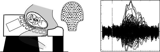
|
|
|
|
|
|
|
|
BIOMAGNETISM |
247 |
|
|
|
|
30 |
stim. |
|
|
|
|
|
|
|
|
(fT) |
20 |
|
|
|
|
|
|
|
Sensors |
(b) |
amplitude |
10 |
|
|
|
|
|
|
|
References |
|
|
|
|
|
|
|
|
|
|
|
Sensor array |
Signal |
0 |
|
|
|
|
|
|
|
|
|
|
|
|
|
|
|
|
||
|
|
|
|
|
|
|
|
|
|
|
|
|
|
–10 |
|
|
|
|
|
|
|
|
|
|
(c) |
|
|
|
|
|
|
|
|
|
|
–20 |
|
|
|
|
|
|
|
|
(a) |
|
–0.2 |
0 |
0.2 |
0.4 |
0.6 |
0.8 |
1 |
|
|
|
|
|
|
Time (s) |
|
|
|
|
|
|
|
|
|
|
|
|
|
|
|
|
Figure 16. Dedicated system for fetal MEG measurement. (a) Schematic diagram of SQUID Array for Reproductive Assessment (SARA) (52). (b) Layout of 151 sensing channels. (c) Example of flash evoked fMEG response, overlay of 151 SARA channels. The fetus with gestation age of 28 weeks was stimulated by 33 ms duration flashes of 625 nm wavelength light (220). Vertical dashed line corresponds to the flash stimulus onset. (Adapted from Ref. 221).
relatively large, up to 500 fT, and can represent interference during evoked fMEG responses.
Early fMEG experiments used single or multiple-chan- nel probes with relatively small area of coverage, requiring a search for the region with the largest signals. Recently, a dedicated fetal MEG system, the SQUID Array for Reproductive Assessment (SARA), was constructed and operated (52). The SARA system consists of an array of 151 SQUID sensors covering the mother’s anterior abdominal surface in late gestation, from the perineum to the top of the uterus as shown in Fig. 16a and b. The primary sensor flux transformers are axial first-order gradiometers, with 8 cm baseline with a nominal SQUID sensor noise density of 4 fT/Hz1/2. The SARA system is now being used routinely and was recently used to measure the first fetal visual evoked field to high intensity light stimuli presented to the maternal abdomen (220). An example of a flash evoked response from the fetal brain is shown in Fig. 16c.
Other Applications
Biosusceptometry. The greatest interest in biosusceptometry has stemmed from its potential to assess noninvasively iron overload in the human liver. This potentially fatal condition arises in individuals with hemoglobinopathies that require frequent blood transfusions (e.g., sickle cell anemia) or involve abnormal production of hemoglobin (hemachromatosis and beta-thalassemia). Standard methods for assessing iron overload can be highly invasive (e.g., liver biopsy) and biosusceptometry offers a safer and potentially more accurate diagnostic tool. Iron, which is normally strongly ferromagnetic, is stored in the liver bound by the proteins ferritin and hemosiderin and exhibits a strong paramagnetic response. As a result, measurement of the magnetic moment produced by placing the liver in a uniform magnetic field will be proportional to the total amount of iron in the liver: a method known as biomagnetic liver susceptometry (BLS). The basis for this technique was
first proposed and the first measurements carried out in the late 1970s (222).
Most approaches to the measurement of hepatic iron concentration involve placing the patient’s abdomen directly under a magnetic sensor that also contains a field coil that produces a magnetic field, and lowering the patient by a fixed distance to measure the change in field amplitude due to the magnetized liver (Fig. 11). In order to eliminate the effect of the surrounding air, a water-filled bellows is placed between the abdomen and the device to simulate the diamagnetic properties of the other tissues in the body. The main challenge to accurate estimates of hepatic iron content using BLS is the remaining effect of the varying susceptibility of the lungs and air filled compartments in the abdomen. Since this technique requires the application of a dc magnetic field to the body on the order of about 0.1 T, it is a much more invasive technology in comparison to MEG and MCG, and may be contraindicated in patients with implanted medical devices such as pacemakers. A detailed review of the clinical applications of BLS can be found in (223).
Peripheral Nerve Studies. It is known from the pioneering studies of Wikswo and colleagues (70) that the propagation of action potentials in nerve fibers produces quadrupolar like sources that have a rapidly diminishing magnetic field with distance. This is due to the fact that action potentials consist of a traveling wave of depolarization in the axon, followed closely by a wave of repolarization. In addition, due to varying conduction velocities in the peripheral nerves, action potentials in different axons will not necessarily summate to produce coherent synchronous activity. As a result, activation of compound nerve bundles does not produce coherent dipole-like sources as in the case of the neocortex. However, with sufficient signal averaging it is possible to record the magnetic signature of the sensory nerve action potentials noninvasively in the human: a technique
248 BIOMAGNETISM
referred to as magnetoneurography. These measures have been achieved by placing single channel magnetometers or flat arrays of magnetic sensors over the peripheral nerve pathways and electrically stimulating the nerve. The predicted quadrapolar pattern of traveling actions potentials resulting from electrical stimulation of the finger was reported by Hoshiyama et al. (224) using a 12 channel ‘‘micro-SQUID’’ device placed over the wrist. Mackert et al. (225), using a 49 channel flat triangular array of first-order radial gradiometers were able to measure compound action potentials elicited by tibial nerve stimulation in sensory nerves entering the spinal cord at the lower lumbar region, and have recently using this method clinically to demonstrate impaired nerve conduction in the patients with S1 root compression.
Magnetopneumography. Magnetopneumography refers to the measurement of the remanent magnetism of ferromagnetic particles in the lungs. This technique may be used to assess lung contamination encountered in occupations that may involve the inhalation of ferromagnetic dust particles such as arc-welders, coalminers, asbestos, and foundry and steel workers. Similar to liver biosusceptometry, magnetopneumography involves the application of a weak dc magnetic field to the thorax. However, the field is applied for only a short interval in order to produce a remanent magnetization of ferromagnetic material, usually iron oxides such as magnetite. This remanent magnetic field is then measured to assess to total load of ferromagnetic particles in the lung. These measures can be used to evaluate the quantity and clearance rates of these substances (226,227). A related measure is relaxation: the decay of the remanent field due to the reorientation of the magnetic particles away from their aligned state after application of the dc field. Relaxation times are thought to reflect cellular processes in the lung associated with clearance or macrophage activity on the foreign particles. Recent studies have used magnetopneumography to study the effect of smoking on clearance times of inhaled magnetic particles (228).
Gastrointestinal System. Biomagnetic measurements have also been applied to other areas of the human body. The human gastrointestinal system produces electrical activity associated with the processes of peristalsis and digestion of food. For example, slow electrical activity at frequencies of 3 cycles/min (0.05 Hz) can be recorded from the human stomach using cutaneous surface electrodes or magnetically: a technique referred to as magnetogastrography (MGG). This activity arises from the smooth muscle of the stomach and the detection of changes in frequency with time has been proposed as a method of characterizing gastric disorders (229). Another novel application of biomagnetic instrumentation to gastrointestinal function, is the 3D tracking of the transport of magnetic materials through the gut. This technique has been termed magnetic marker monitoring (MMM) and can be used to monitor the passage and disintegration (by measuring decrease in magnetic moment) of magnetically
labeled pharmaceutical substances through the gastrointestinal system (230).
FUTURE DIRECTIONS
Since its inception 40 years ago with the first recording of the magnetic field of the heart, the field of biomagnetism has expanded immensely to become a major field of basic and applied research. The field of magnetoencephalography, or MEG, has in recent years become a recognized neuroimaging technique, with the development of advanced instruments for the measurement of the electrical activity of the brain with exquisite temporal and spatial resolution. Biomagnetic instrumentation is now at a mature state, with commercially developed measurement systems available for a variety of biomagnetic applications. For example, whole head MEG systems are installed worldwide in >100 research laboratories and clinical centres and are now being used in routine clinical diagnostic procedures. Nevertheless, there remain many areas for further improvement of both instrumentation and data analysis approaches and techniques. In terms of instrumentation, biomagnetometer systems with increased number of sensing channels and capable of unshielded operation will likely be developed, and present systems that require frequent refilling with liquid Helium may be replaced by systems with longer hold times and less frequent cryogen replenishment. The latter may be accomplished either by incorporation of cryocoolers, or the use of sensors that do not require liquid He. The last two technical innovations, combined with production of larger numbers of MEG systems will also help reduce the cost of these instruments.
The analysis and interpretation of biomagnetic measurements is possibly the most significant area for continued research and development, and much progress has been made in the implementation of new signal processing algorithms for the extraction of biomagnetic signals, or improving the spatial resolution of source localization methods. There has been recent interest in combining MEG with its high temporal resolution and other functional imaging techniques such as functional MRI. In addition, advanced image processing techniques, such as the automated extraction of the cortical surface of the brain from structural MRI, will allow the use of more precise physical models of biomagnetic sources. Combination of MEG with its counterpart EEG may also help to develop more accurate models of brain activity. These advancements will aid the development of new clinical applications of biomagnetism such as the use of MEG to study psychiatric disorders, or to study the effects of drug treatments on brain processes related to cognitive deficits, or gain insight into the physiological mechanisms underlying various brain disorders in children, for example, learning disabilities, dyslexia, and autism. Finally, novel applications of biomagnetic measurements, for example, the measurement of heart and brain activity in the fetus, will lead to new applications of biomagnetism in clinical medicine and will further drive the development of improved technology. In sum, biomagnetism will continue
to grow as a novel and powerful noninvasive technique for the study of physiological processes in humans in both health and disease.
BIBLIOGRAPHY
Cited References
1.Baule GM, McFee R. Detection of the magnetic field of the heart. Am Heart J 1963;66:95–96.
2.Cohen D. Magnetoencephalography: evidence of magnetic fields produced by alpha-rhythm currents. Science 1968; 161:784–786.
3.Josephson BD. Possible new effect in superconductive tunneling. Phys Lett 1962;1:251–253.
4.Zimmerman JE. Recent developments in superconducting devices. J Appl Phys 1971;42:30–37.
5.Cohen D, Edelsack EA, Zimmerman JE. Magnetocardiograms taken inside a shielded room with a superconducting pointcontact magnetometer. Appl Phys Lett 1970;16:278–280.
6.Cohen D. Magnetoencephalography: detection of the brain’s electrical activity with a superconducting magnetometer. Science 1972;175:664–666.
7.Cheyne D, Vrba J, Crisp D, Betts K, Burbank M, Cheung T, Fife A, Haid G, Kubik P, Lee S, McCubbin J, McKay J, McKenzie D, Spear P, Taylor B, Tillotson M, Weinberg H, Basar E. Use of an unshielded, 64 channel, whole cortex MEG system in the study of normal and pathological brain function. Proceedings of the Satellite Symposium on Neuroscience and Technology, 14th Annu Conf IEEE Eng Med Biol Soc Lyon. France: 1992; 46–50.
8.Ahonen AI, Ha¨ma¨la¨inen MS, Kajola MJ, Knuutila JET, Laine PP, Lounasmaa OV, Simola JT, Tesche CD, Vilkman VA. A 122-channel magnetometer covering the whole head. Proceedings of the Satellite Symposium on Neuroscience and Technology, 14th Annu Conf IEEE Eng Med Biol Soc Lyon. France: 1992; 16–20.
9.Clarke J. SQUIDs: theory and practice. In: Weinstock H, Ralston RW, editors. The New Superconducting Electronics. Dordrecht, Boston: Kluwer Academic; 1993. p 123–180.
10.Vrba J, Robinson SE. Signal processing in magnetoencephalography. Methods 2001;25:249–271.
11.Jaklevic R, Lambe RC, Silver AH, Mercereau JE. Quantum interference effects in Josephson tunneling. Phys Rev Lett 1964;12:159–160.
12.Jaycox JM, Ketchen MB. Planar coupling scheme for ultra low noise dc SQUIDs. IEEE Trans Magn 1981;MAG-17:400– 403.
13.Ketchen MB, Jaycox JM. Ultra low noise tunnel junction dc SQUID with a tightly coupled planar input coil. Appl Phys Lett 1982;40:736–738.
14.Clarke J, Goubau WM, Ketchen MB. Tunnel junction DC SQUID: fabrication, operation, and performance. J Low Temp Phys 1976;25:99–144.
15.McKay J, Vrba J, Betts K, Burbank MB, Lee S, Mori K, Nonis D, Spear P, Uriel Y. Implementation of multichannel biomagnetic measurement system using DSP technology. Proc Can Conf Elect Comp Eng 1993; 1090–1093.
16.Robinson SE. A digital SQUID controller for unshielded biomagnetic measurement. In: Aine C, Okada Y, Stroink G, Swithenby S, Wood C, editors. Biomag96: Proc 10th Int Conf Biomag; 2000; New York: Springer; p 103– 106.
17.Knuutial JET, Ahonen AI, Hamalainen MS, Kajola MJ, Petteri Laine P, Lounasmaa OV, Parkkonen LT, Simola JTA, Tesche CD. A 122-channel whole-cortex SQUID system
BIOMAGNETISM 249
for measureing the brain’s magnetic fields. IEEE Trans Mag 1993;29:3315–3321.
18.Vrba J. Multichannel SQUID biomagnetic systems. In: Weinstock H, editor. Applications of Superconductivity. Dordrecht: Kluwer Academic Publishers; 2000. p 61–138.
19.Kominis IK, Kornack TW, Allred JC, Romalis MV. A subfemtotesla multichannel atomic magnetometer. Nature (London) 2003;422:596–599.
20.Zimmerman JE. SQUID instruments and shielding for low level magnetic measurements. J Appl Phys 1977;48:702– 710.
21.H. G. Vacuumschmelze GmbH, Shielded room model AK-3.
22.Sullivan GW, Flynn ER. Performance of the Los Alamos Shielded Room. In: Atsumi K, Kotani M, Ueno S, Katila T, Williamson SJ, editors. Biomagnetism ‘87. Tokyo: Tokyo Denki University Press; 1987. p 486–489.
23.Erne´ SN, Hahlbohm HD, Scheer G, Trontelj Z. The Berlin magnetically shielded room (BMSR). In: Erne´ SN, editor. Biomagnetism. Berlin: Walter de Gruyter; 1981. p 79–87.
24.Bork J, Hahlbohm HD, Klein R, Schnabel A. The 8-layered magnetically shielded room of the PTB: Design and construction. In: Nenonen J, Ilmoniemi R, Katila T, editors. Biomag 2000. Proc 12th Int Conf Biomag. Espoo, Finland: Helsinki University of Technology; 2001. p 970–973.
25.Matsuba H, Shintomi K, Yahara A, Irisawa D, Imai K, Yoshida H, Seike S. Superconducting shielding enclosing a human body for biomagnetic measurement. In: Baumgartner C, Deecke L, Stroink G, Williamson SJ, editors. Biomagnetism: Fundamental research and clinical applications. Amsterdam, The Netherlands: Elsevier Science, IOS Press; 1995. p 483–489.
26.Matsumoto K, Yamagishi Y, Wakusawa A, Noda T, Fujioka K, Kuraoka Y. SQUID based active shield for biomagnetic measurements. In: Hoke M, Erne´ SN, Okada Y, Romani Gl, editors. Biomagnetism: clinical aspects. Proc 8th Int Conf Biomag. Amsterdam: Excerpta Medica; 1992. p 857– 861.
27.Malmivuo J, Lekkala J, Kontro P, Suomaa I, Vihinin H. Improvement of the properties of an eddy current magnetic shield with active compensation. J Phys E: Sci Instr 1987;20:151–164.
28.ter Brake HJM, Wieringa HJ, Rogalla H. Improvement of the performance of a m-metal magnetically shielded room by means of active compensation. Meas Sci Technol 1991;2: 596–601.
29.Vrba J. SQUID gradiometers in real environments. In: Weinstock H, editor. SQUID sensors: Fundamentals, Fabrication, and Applications. Dordrecht, Boston: Kluwer Academic Publishers; 1996. p 117–178.
30.Vrba J, Robinson SE. SQUID sensor array configurations for magnetoencephalography applications. Supercond Sci Technol 2002;15:R51–R89.
31.Vrba J. Magnetoencephalography: the art of finding a needle in a haystack. Phys C 2002;368:1–9.
32.Huotilainen M, Ilmoniemi RJ, Tiitinen H, Lavikainen J, Alho K, Kajola M, Naatanen R. The projection method in removing eye blink artefacts from multichannel MEG measurements.
In: Baumgartner C, Deecke L, Stroink G, Williamson SJ, editors. Biomagnetism: Fundamental research and clinical applications. Elsevier Science, IOS Press; 1995.
p 363–367.
33.Tesche CD, Uusitalo MA, Ilmoniemi RJ, Huotilainen M, Kajola M, Salonen O. Signal-space projections of MEG data characterize both distributed and well-localized neuronal sources. Electroencephalogr Clin Neurophys 1995; 95:189–200.
250BIOMAGNETISM
34.Uusitalo MA, Ilmoniemi RJ. Signal-space projection method for separating MEG or EEG into components. Med Biol Eng Comput 1997;35:135–140.
35.Parkkonen LT, Simola JT, Tuoriniemi JT, Ahonen AI. An interference suppression system for multichannel magnetic field detector arrays. In: Yoshimoto T, Kotani M, Kuriki S, Karibe H, Nakasato N, editors. Recent Advances in Biomagnetism. Sendai: Tohoku University Press; 1999. p 13–16.
36.Taula S, Kajola MJ, Simola JT. The Signal Space Separation method. 14th Conf Int Soc Brain Electromagnetic Topography. Santa Fe, NM; 2003.
37.Ioannides AA, Mu¨ tter J, Barna-Popescu EA. Irreducible tensor representation of MEG signals: Theory and applications. In: Nenonen J, Ilmoniemi R, Katila T, editors. Biomag 2000. Proc 12th Int Conf Biomag. Espoo, Finland: Helsinki University of Technology; 2001. p 883–886.
38.ter Brake HJM. Cryogenic systems for superconducting devices. In: Weinstock H, editor. Applications of superconductivity. Dordrecht: Kluwer Academic Publishers; 2000. p 561–639.
39.VSM MedTech Ltd. (CTF) 9 Burbidge St. Coquitlam, B.C., Canada (www.vsmmedtech.com).
40.Nowak H. Biomagnetic Instrumentation. In: Andra¨ W, Nowak H, editors. Magnetism in Medicine. Berlin: Wiley VCH; 1998. p 88–135.
41.Hoenig HE, Daalmans GM, Ba¨r L, Bo¨mmel F, Paulus A, Uhl D, Weisse HJ, Schneider S, Seifert H, Reichenberger H, Abraham-Fuchs K, Multichannel DC. SQUID sensor array for biomagnetic applications. IEEE Trans Magn 1991; 27:2777–2785.
42.Tsukada K, Kandori A, Miyashita T, Sasabuchi H, Suzuki H, Kondo S, Komiyama Y, Teshogawara K. A simplified superconducting quantum interference device system to analyze
vector components of a cardiac magnetic field. Proc 20th Annu Int Conf IEEE/EMBS. Hong Kong; 1998.
p 524–527.
43.Van Leeuwen P, Haupt C, Hoormann C, Hailer B, Mackert BM, Stroink G. A 67 channel biomagnetometer designed for cardiology and other applications. In: Yoshimoto T, Kotani M, Kuriki S, Karibe H, Nakasato N, editors. Recent Advances in Biomagnetism. Sendai: Tohoku University Press; 1999. p 89– 92.
44.Erne´ SN, Pasquarelli A, Kammrath H, Della Penna S, Torquati K, Pizzella V, Rossi R, Granata C, Russo M. Argos 55 - the new MCG system in Ulm. In: Yoshimoto T, Kotani M, Kuriki S, Karibe H, Nakasato N, editors. Recent Advances in Biomagnetism. Sendai: Tohoku University Press; 1999. p 27– 30.
45.Montonen J, Ahonen A, Ha¨ma¨la¨inen M, Ilmoniemi R, Laine P, Nenonen J, Paavola M, Simelius K, Simola J, Katila T. Magnetocardiographic functional imaging studies in BioMag Laboratory. In: Aine CJ, Okada Y, Stroink G, Swithenby S, Wood C, editors. Biomag 96: Proc Tenth Int Conf Biomag. New York: Springer; 2000. p 494–497.
46.ter Brake HJM, Janssen N, Flokstra J, Veldhuis D, Rogalla H. Multichannel heart scanner based on high-Tc SQUIDs. IEEE Trans Appl Supercond 1997;7:2545–2548.
47.Seidel P, Schmidl F, Wunderlich S, Do¨rrer L, Vogt T, Schneidewind H, Weidl R, Lo¨sche R, Leder U, Solbig O, Nowak H. High-Tc SQUID systems for practical use. IEEE Trans Appl Supercond 1999;9:4077–4080.
48.Kouznesov KA, Borgmann J, Clarke CJS. High-Tc secondorder gradiometer for magnetocardiography in an unshielded environment. Appl Phys Lett 1999;75:1979–1981.
49.Zhang Y, Panaitov G, Wang SG, Wolters N, Otto R, Schubert J, Zander W, Krause HJ, Soltner H, Bousack H, Braginski A.
Second-order, high-temperature superconducting gradiometer for magnetocardiography in an unshielded environment. Appl Phys Lett 2000;76:906–908.
50.Ludwig F, Jansman ABM, Drung D, Lindstro¨m M, Bechstien S, Beyer J, Flokstra J, Schurig T. Optimization of directcoupled high-Tc SQUID magnetometers for operation in a magnetically shielded environment. IEEE Trans Appl Supercond 2001;11:1824–1827.
51.Barthelmess H-J, Halverscheid M, Schiefenho¨vel B, Heim E, Schilling M, Zimmerman R. Low-noise biomagnetic measurements with a multichannel dc-SQUID system at
77 K. IEEE Trans Appl Supercond 2001;11:657–
660.
52.Robinson SE, BM, FA, HG, KP, I Sekachev, Taylor B, Tillotson M, Wong VJG, Lowery C, Eswaran H, Wilson D, Murphy P, Preissl H. A biomagnetic instrument for human reproductive assessment. In: Nenonen J, Ilmoniemi R, Katila T, editors. Biomag2000, Proc 12th Int Conf Biomag. Espoo, Finland: Helsinki University of Technology; 2001. p 919– 922.
53.4-D Neuroimaging Inc. 9727 Pacific Heights Blvd., San Diego, CA 92121-3719 (www.4dneuroimaging.com).
54.Neuromag Oy, P.O. Box 68, FIN-00511 Helsinki, Finland (www.neuromag.com).
55.Eagle Technology, Inc. 1-2-23 Hirosaka, Kanazawa Ishikawa 920-0962, Japan (www.eagle-tek.com).
56.Advanced Technologies Biomagnetics S.r.l, Via Martiri di Pietransieri 2, 65129 Pescara, Italy (www.atb-it.com).
57.Polhemus Inc., Hercules Drive, P.O. Box 560, Colchester, VT 05446.
58.Bramidis PD, Ioannides AA. Combination of point and surface matching techniques for accurate registration of MEG and MRI. In: Aine CJ, Okada Y, Stroink G, Swithenby S, Wood C, editors. Biomag 96: Proc 10th Int Conf Biomag. New York: Springer; 1997. p 1126–1129.
59.Abraham-Fuchs K, Lindner L, Weganer P, Nestel F, Schneider S. Fusion of biomagnetism with MRI or CT images by contour fitting. Biomed Eng 1991;36(Suppl.): 88–89.
60.Kober H, Nimsky C, Vieth J, Fahlbusch R, Ganslandt O. Coregistration of function and anatomy in frameless stereotaxy by contour fitting, Stereotact Funct. Neurosurg 2002;79:272– 283.
61.Braginski A, Krause HJ, Vrba J. SQUID magnetometers. In: Francombe MH, editor. Handbook of Thin Film Devices, Volume 3: Superconducting Film Devices. San Diego: Academic Press; 2000. p 149–225.
62.Farrell DE, Tripp JH, Zanzucchi PE. Magnetic measurements of human iron stores. IEEE Transactions on Magnetics May-1980;16:818–823.
63.Paulson DN, Fagaly RL, Toussaint RM, Fischer R. Biomagnetic susceptometer with SQUID instrumentation. IEEE Trans Magn 1991;27:3249–3252.
64.Fischer F. Liver iron susceptometry. In: Andra¨ W, Nowak H, editors. Magnetism in medicine: a handbook. Berlin; New
York: Wiley-VCH; 1998. p 286–301.
¨
65. Helmholtz H. Uber einige Gesetze der Vertheilung elektrischer Stro¨me in ko¨perlichen Leitern mit Anwendung auf die thierisch-elektrischen Versuche. Ann Phys Chem 1853;89:211–233, 353–377.
66. Ha¨ma¨la¨inen M, Hari R, Ilmoniemi RJ, Knuutila JET, Lounasmaa OV. Magnetoencephalography-theory, instrumentation, and applications to noninvasive studies of the working human brain. Rev Mod Phys 1993;65:413–497.
67.Jeffs B, Leahy R, Singh M. An evaluation of methods for neuromagnetic image reconstruction. IEEE Trans Biomed Eng 1987;34:713–723.
68.Baillet S, Mosher JC, Leahy R. Electromagnetic brain mapping. IEEE Signal Proc Mag 2001;18:14–30.
69.Mosher JC, Leahy RM, Lewis PS. EEG and MEG: forward solutions for inverse methods. IEEE Trans Biomed Eng 1999;46:245–259.
70.Wikswo JP, Barach JP, Freeman JA. Magnetic field of a nerve impulse: first measurements. Science 1980;208:53–55.
71.Swinney KR, Wikswo, Jr. JP. A calculation of the magnetic field of a nerve action potential. Biophys J 1980;32:719–731.
72.Tesche CD. Non-invasive imaging of neuronal population dynamics in human thalamus. Brain Res 1996;729:253– 258.
73.Tesche CD, Karhu J, Tissari SO. Non-invasive detection of neuronal population activity in human hippocampus. Brain Res Cogn Brain Res 1996;4:39–47.
74.Humphrey DR. Re-analysis of the antidromic cortical response. II. On the contribution of cell discharge and PSPs to the evoked potentials. Electroencephalogr Clin Neurophysiol 1968;25:421–442.
75.Creutzfeldt OD, Watanabe S, Lux HD. Relations between EEG phenomena and potentials of single cortical cells. I. Evoked responses after thalamic and epicortical stimulation. Electroencephalogr Clin Neurophysiol 1966;20:1–18.
76.Mitzdorf U. Current source-density method and application in cat cerebral cortex: investigation of evoked potentials and EEG phenomena. Physiol Rev 1985;65:37–100.
77.Okada YC, Wu J, Kyuhou S. Genesis of MEG signals in a mammalian CNS structure. Electroencephalogr Clin Neurophysiol 1997;103:474–485.
78.Okada Y. Toward understanding the physiological origins of neuromagnetic signals. In: Lu Z-L, Kaufman L, editors. Magnetic Source Imaging of the Brain. Mahwah. New Jersey: Lawrence Erlbaum Associates; 2003. p 43–76.
79.Weinberg H, Brickett P, Coolsma F, Baff M. Magnetic localisation of intracranial dipoles: simulation with a physical model. Electroencephalogr Clin Neurophysiol 1986;64:159– 170.
80.Cheyne D, Roberts LE, Gaetz W, Bosnyak D, Nahmias C, Christoforou N, Weinberg H. Somatotopic organization of human somatosensory cortex: a comparison of EEG, MEG and fMRI methods. In: Koga Y, Nagata K, Hirata K, editors. Brain Topography Today. Amsterdam: Elsevier Science; 1998. p 76–81.
81.Sarvas J. Basic mathematical and electromagnetic concepts of the biomagnetic inverse problem. Phys Med Biol 1987;32: 11–22.
82.Hillebrand A, Barnes GR. A quantitative assessment of the sensitivity of whole-head MEG to activity in the adult human cortex. Neuroimage 2002;16:638–650.
83.Lu ZL, Williamson SJ. Spatial extent of coherent sensoryevoked cortical activity. Exp Brain Res 1991;84:411–416.
84.Ha¨ma¨la¨inen MS, Ilmoniemi RJ. Interpreting measured magnetic fields of the brain: Estimates of current distribution. Report TKK-F-A559. Helsinki University of Technology: Espoo, Finland, 1984.
85.Scherg M, Von Cramon D. Two bilateral sources of the late AEP as identified by a spatio-temporal dipole model. Electroencephalogr Clin Neurophysiol 1985;62:32–44.
86.Huang MX, Mosher JC, Leahy RM. A sensor-weighted over- lapping-sphere head model and exhaustive head model comparison for MEG. Phys Med Biol 1999;44:423–440.
87.Gorodnitsky IF, George JS, Rao BD. Neuromagnetic source imaging with FOCUSS: a recursive weighted minimum norm algorithm. Electroencephalogr Clin Neurophysiol 1995;95: 231–251.
88.Wagner M, Wischmann HA, Fuchs M, Kohler T, Drenckhahn R. Current density reconstruction using the L1 norm. In:
BIOMAGNETISM 251
Aine CJ, Okada Y, Stroink G, Swithenby S, Wood C, editors. Biomag96. New York: Springer-Verlag; 2000. p 393–396.
89.Ioannides AA, Bolton JPR, Clarke CJS. Continuous probabilistic solutions to the biomagnetic inverse problem. Inverse Problems 1990;6:523–542.
90.Pascual-Marqui RD, Michel CM, Lehmann D. Low resolution electromagnetic tomography: a new method for localizing electrical activity in the brain. Int J Psychophysiol 1994; 18:49–65.
91.David O, Garnero L, Cosmelli D, Varela FJ. Estimation of neural dynamics from MEG/EEG cortical current density maps: application to the reconstruction of large-scale cortical synchrony. IEEE Trans Biomed Eng 2002;49: 975–987.
92.Baillet S, Garnero L. A Bayesian approach to introducing anatomo-functional priors in the EEG/MEG inverse problem. IEEE Trans Biomed Eng 1997;44:374–385.
93.Schmidt DM, George JS, Wood CC. Bayesian inference applied to the electromagnetic inverse problem. Hum Brain Mapp 1999;7:195–212.
94.Ha¨ma¨la¨inen MS, Haario H, Lehtinen MS. Inferences about sources of neuromagnetic fields using Bayesian parameter estimation. Espoo, Finland: Helsinki University of Technolgy; 1987.
95.Sorenson HW. Parameter estimation. New York: Marcel Dekker; 1980.
96.Robinson SE, Rose DF. Current source estimation by spatially filtered MEG. In: HokeM, Erne´ SN, Okada Y, Romani GL, editors. Biomagnetism: clinical aspects. Proc 8th Int Conf Biomag. Amsterdam: Excerpta Medica; 1992. p 761–765.
97.Frost OL. An algorithm for linearly constrained adaptive array processing. Proc IEEE 1972;60:926–935.
98.Van Veen B, Buckley K. Beamforming: A versatile
approach to spatial filtering, in IEEE ASSP Mag.; 1988. p 4–24.
99.Godara LC. Application of antenna array to mobile communications, Part II: Beam-Forming and direction-of-arrival considerations. Proc IEEE 1997;85:1195–1245.
100.Van Veen BD, Van Drongelen W, Yuchtman M, Suzuki A. Localization of brain electrical activity via linearly constrained minimum variance spatial filtering. IEEE Trans Biomed Eng 1997;44:867–880.
101.Robinson SE, Vrba J. Functional neuroimaging by synthetic aperture magnetometry (SAM). In: Yoshimoto T, Kotani M,
Kuriki S, Karibe H, Nakasato N, editors. Recent Advances in Biomagnetism. Sendai: Tohoku University Press; 1999.
p 302–305.
102.Vrba J, Robinson SE. Linearly constrained minimum variance beamformers, synthetic aperture magnetometry and MUSIC in MEG applications. IEEE, Proc 34th Asilomar Conf. Signals, Systems, Comput. Pacific Grove, CA: Omnipress; 2000. p 313–317.
103.Schmidt RO. Multiple emitter location and signal parameter estimation. IEEE Trans Anten Propagat 1986;AP-34:276– 280.
104.Mosher JC, Lewis PS, Leahy RM. Multiple dipole modeling and localization from spatio-temporal MEG data. IEEE Trans Biomed Eng 1992;39:541–557.
105.Mosher JC, Leahy R. Source localization using recursively applied and projected (RAP) MUSIC. IEEE Trans Signal Proc 1999;47:332–340.
106.Maier J, Dagnelie G, Spekreijse H, van Dijk BW. Principal components analysis for source localization of VEPs in man. Vision Res 1987;27:165–177.
107.Achim A, Richer F, Saint-Hilaire JM. Methods for separating temporally overlapping sources of neuroelectric data. Brain Topogr 1988;1:22–28.
252 BIOMAGNETISM
108.Jung TP, Makeig S, Mckeown MJ, Bell AJ, L. T, Sejnowski TJ. Imaging brain dynamics using independent component analysis. Proc IEEE 2001;89:1107–1122.
109.Cardoso J-F. Blind signal separation: Statistical principles. Proc IEEE 1998;86:2009–2025.
110.Hyvarinen A. Fast and robust fixed-point algorithms for independent component analysis. IEEE Trans Neural Networks 1999;10:626–634.
111.Makeig S, Jung TP, Bell AJ, Ghahremani D, Sejnowski TJ. Blind separation of auditory event-related brain responses into independent components. Proc Natl Acad Sci USA 1997;94:10979–10984.
112.Ziehe A, Muller KR, Nolte G, Mackert BM, Curio G. Artifact reduction in magnetoneurography based on time-delayed second-order correlations. IEEE Trans Biomed Eng 2000; 47:75–87.
113.Lewine JD, Orrison, Jr. WW. Magnetic source imaging: basic principles and applications in neuroradiology. Acad Radiol 1995;2:436–440.
114.Wheless JW, Castillo E, Maggio V, Kim HL, Breier JI, Simos PG, Papanicolaou AC. Magnetoencephalography (MEG) and magnetic source imaging (MSI). Neurologist 2004; 10:138– 153.
115.Lu Z-L, Kaufman L, editors. Magnetic Source Imaging of the Brain. Mahwah, NJ: Lawrence Erlbaum Associates; 2003.
116.Gallen CC, Schwartz BJ, Bucholz RD, Malik G, Barkley GL, Smith J, Tung H, Copeland B, Bruno L, Assam S. Presurgical localization of functional cortex using magnetic source imaging. J Neurosurg 1995;82:988–994.
117.Roberts TP, Poeppel D, Rowley HA. Magnetoencephalography and magnetic source imaging. Neuropsychiat Neuropsychol Behav Neurol 1998;11:49–64.
118.Brenner D, Lipton J, Kaufman L, Williamson SJ. Somatically evoked magnetic fields of the human brain. Science 1978;199:81–83.
119.Kakigi R, Hoshiyama M, Shimojo M, Naka D, Yamasaki H, Watanabe S, Xiang J, Maeda K, Lam K, Itomi K, Nakamura A. The somatosensory evoked magnetic fields. Prog Neurobiol 2000;61:495–523.
120.Nakamura A, Yamada T, Goto A, Kato T, Ito K, Abe Y, Kachi T, Kakigi R. Somatosensory homunculus as drawn by MEG. Neuroimage 1998;7:377–386.
121.Curio G, Mackert BM, Burghoff M, Koetitz R, Abraham-
Fuchs K, Harer W. Localization of evoked neuromagnetic 600 Hz activity in the cerebral somatosensory system. Electroencephalogr Clin Neurophysiol 1994;91:483– 487.
122.Hashimoto I, Mashiko T, Imada T. Somatic evoked highfrequency magnetic oscillations reflect activity of inhibitory interneurons in the human somatosensory cortex. Electroencephalogr Clin Neurophysiol 1996;100:189–203.
123.Ikeda H, Leyba L, Bartolo A, Wang Y, Okada YC. Synchronized spikes of thalamocortical axonal terminals and cortical neurons are detectable outside the pig brain with MEG. J Neurophysiol 2002;87:626–630.
124.Hari R, Karhu J, Ha¨ma¨la¨inen MS, Knuutila J, Salonen O, Sams M, Vilkman V. Functional organization of the human first and second somatosensory cortices: a neuromagnetic study. Eur J Neurosci 1993;5:724–734.
125.Suk J, Ribary U, Cappell J, Yamamoto T, Llinas R. Anatomical localization revealed by MEG recordings of the human somatosensory system. Electroencephalogr Clin Neurophysiol 1991;78:185–196.
126.Flor H, Elbert T, Knecht S, Wienbruch C, Pantev C, Birbaumer N, Larbig W, Taub E. Phantom-limb pain as a perceptual correlate of cortical reorganization following arm amputation. Nature (London) 1995;375:482–484.
127.Elbert T, Pantev C, Wienbruch C, Rockstroh B, Taub E. Increased cortical representation of the fingers of the left hand in string players. Science 1995;270:305–307.
128.Deecke L, Weinberg H, Brickett P. Magnetic fields of the human brain accompanying voluntary movement: Bereitschaftsmagnetfeld. Exp Brain Res 1982;48:144–148.
129.Cheyne D, Weinberg H. Neuromagnetic fields accompanying unilateral finger movements: pre-movement and movementevoked fields. Exp Brain Res 1989;78:604–612.
130.Kristeva R, Cheyne D, Lang W, Lindinger G, Deecke L. Movement-related potentials accompanying unilateral and bilateral finger movements with different inertial loads. Electroencephalogr Clin Neurophysiol 1990;75:410–418.
131.Cheyne D, Endo H, Takeda T, Weinberg H. Sensory feedback contributes to early movement-evoked fields during voluntary finger movements in humans. Brain Res 1997;771:196– 202.
132.Kelso JA, Fuchs A, Lancaster R, Holroyd T, Cheyne D, Weinberg H. Dynamic cortical activity in the human brain reveals motor equivalence. Nature (London) 1998;392:814– 818.
133.Endo H, Kizuka T, Masuda T, Takeda T. Automatic activation
in the human primary motor cortex synchronized with movement preparation. Cogn Brain Res 1999;8:229–239.
134.Xiang J, Hoshiyama M, Koyama S, Kaneoke Y, Suzuki H, Watanabe S, Naka D, Kakigi R. Somatosensory evoked magnetic fields following passive finger movement. Brain Res Cogn Brain Res 1997;6:73–82.
135.Lang W, Cheyne D, Hollinger P, Gerschlager W, Lindinger G. Electric and magnetic fields of the brain accompanying internal simulation of movement. Cogn Brain Res 1996;3:125–129.
136.Conway BA, Halliday DM, Farmer SF, Shahani U, Maas P, Weir AI, Rosenberg JR. Synchronization between motor cortex and spinal motoneuronal pool during the performance of a maintained motor task in man. J Physiol 1995;489(Pt. 3): 917–924.
137.Brown P. Cortical drives to human muscle: the Piper and related rhythms. Prog Neurobiol 2000;60:97–108.
138.Salenius S, Avikainen S, Kaakkola S, Hari R, Brown P. Defective cortical drive to muscle in Parkinson’s disease and its improvement with levodopa. Brain 2002;125: 491– 500.
139.Timmermann L, Gross J, Dirks M, Volkmann J, Freund HJ, Schnitzler A. The cerebral oscillatory network of parkinsonian resting tremor. Brain 2003;126:199–212.
140.Hari R, Salmelin R. Human cortical oscillations: a neuromagnetic view through the skull. Trends Neurosci 1997;20: 44– 49.
141.Cheyne D, Gaetz W, Garnero L, Lachaux JP, Ducorps A, Schwartz D, Varela FJ. Neuromagnetic imaging of cortical oscillations accompanying tactile stimulation. Brain Res Cogn Brain Res 2003;17:599–611.
142.Feige B, Kristeva-Feige R, Rossi S, Pizzella V, Rossini PM. Neuromagnetic study of movement-related changes in rhythmic brain activity. Brain Res 1996;734:252–260.
143.Gaetz WC, Cheyne DO. Localization of human somatosensory cortex using spatially filtered magnetoencephalography. Neurosci Lett 2003;340:161–164.
144.Taniguchi M, Kato A, Fujita N, Hirata M, Tanaka H, Kihara T, Ninomiya H, Hirabuki N, Nakamura H, Robinson SE, Cheyne D, Yoshimine T. Movement-related desynchronization of the cerebral cortex studied with spatially filtered magnetoencephalography. Neuroimage 2000;12:298–306.
145.Brenner D, Williamson SJ, Kaufman L. Visually evoked magnetic fields of the human brain. Science 1975;190:480–482.
146.Supek S, Aine CJ, Ranken D, Best E, Flynn ER, Wood CC. Single vs. paired visual stimulation: superposition of early
neuromagnetic responses and retinotopy in extrastriate cortex in humans. Brain Res 1999;830:43–55.
147.Fylan F, Holliday IE, Singh KD, Anderson SJ, Harding GF. Magnetoencephalographic investigation of human cortical area V1 using color stimuli. Neuroimage 1997;6:47–57.
148.Singh KD, Barnes GR, Hillebrand A, Forde EM, Williams AL. Task-related changes in cortical synchronization are spatially coincident with the hemodynamic response. Neuroimage 2002;16:103–114.
149.Anderson SJ, Holliday IE, Singh KD, Harding GF. Localization and functional analysis of human cortical area V5 using magneto-encephalography. Proc R Soc London Sev B Biol Sci 1996;263:423–431.
150.Maruyama K, Kaneoke Y, Watanabe K, Kakigi R. Human cortical responses to coherent and incoherent motion as measured by magnetoencephalography. Neurosci Res 2002;44:195–205.
151.Anderson SJ, Holliday IE, Harding GF. Assessment of cortical dysfunction in human strabismic amblyopia using magnetoencephalography (MEG). Vision Res 1999;39:1723–1738.
152.Reite M, Edrich J, Zimmerman JT, Zimmerman JE. Human magnetic auditory evoked fields. Electroencephalogr Clin Neurophysiol 1978;45:114–117.
153.Romani GL, Williamson SJ, Kaufman L, Brenner D. Characterization of the human auditory cortex by the neuromagnetic method. Exp Brain Res 1982;47:381–393.
154.Pantev C, Hoke M, Lehnertz K, Lutkenhoner B, Anogianakis G, Wittkowski W. Tonotopic organization of the human auditory cortex revealed by transient auditory evoked magnetic fields. Electroencephalogr Clin Neurophysiol 1988;69: 160– 170.
155.Pantev C, Lutkenhoner B. Magnetoencephalographic studies of functional organization and plasticity of the human auditory cortex. J Clin Neurophysiol 2000;17:130–142.
156.Roberts TP, Ferrari P, Stufflebeam SM, Poeppel D. Latency of the auditory evoked neuromagnetic field components: stimulus dependence and insights toward perception. J Clin Neurophysiol 2000;17:114–129.
157.Weinberg H, Cheyne D, Brickett P, Harrop R, Gordon R. An interaction of cortical sources associated with simultaneous auditory and somatosensory stimulation. In: Pfurtscheller G, Lopes da Silva FH, editors. Functional Brain Imaging. Lewiston, N.Y.: Hans Huber Publishers; 1988. p 83–88.
158.Ribary U, Ioannides AA, Singh KD, Hasson R, Bolton JP, Lado F, Mogilner A, Llinas R. Magnetic field tomography of coherent thalamocortical 40-Hz oscillations in humans. Proc Natl Acad Sci USA 1991;88:11037–11041.
159.Ross B, Picton TW, Pantev C. Temporal integration in the human auditory cortex as represented by the development of the steady-state magnetic field. Hear Res 2002;165:68–84.
160.Starr A, Kristeva R, Cheyne D, Lindinger G, Deecke L. Localization of brain activity during auditory verbal shortterm memory derived from magnetic recordings. Brain Res 1991;558:181–190.
161.Mecklinger A, Maess B, Opitz B, Pfeifer E, Cheyne D, Weinberg H. A MEG analysis of the P300 in visual discrimination tasks. Electroencephalogr Clin Neurophysiol 1998;108:45– 56.
162.Alho K. Cerebral generators of mismatch negativity (MMN) and its magnetic counterpart (MMNm) elicited by sound changes. Ear Hear 1995;16:38–51.
163.Halgren E, Raij T, Marinkovic K, Jousmaki V, Hari R. Cognitive response profile of the human fusiform face area as determined by MEG. Cereb Cortex 2000;10:69–81.
164.Salmelin R, Hari R, Lounasmaa OV, Sams M. Dynamics of brain activation during picture naming. Nature (London) 1994;368:463–465.
BIOMAGNETISM 253
165.Sams M, Aulanko R, Hamalainen M, Hari R, Lounasmaa OV, Lu ST, Simola J. Seeing speech: visual information from lip movements modifies activity in the human auditory cortex. Neurosci Lett 1991;127:141–145.
166.Pulvermuller F, Shtyrov Y, Ilmoniemi R. Spatiotemporal dynamics of neural language processing: an MEG study using minimum-norm current estimates. Neuroimage 2003;20:1020–1025.
167.Pylkkanen L, Marantz A. Tracking the time course of word recognition with MEG. Trends Cogn Sci 2003;7:187–189.
168.Roberts TP, Ferrari P, Poeppel D. Latency of evoked neuromagnetic M100 reflects perceptual and acoustic stimulus attributes, Neuroreport 1998;9:3265–3269.
169.Helenius P, Salmelin R, Service E, Connolly JF. Semantic cortical activation in dyslexic readers. J Cogn Neurosci 1999;11:535–550.
170.Salmelin R, Schnitzler A, Schmitz F, Jancke L, Witte OW, Freund HJ. Functional organization of the auditory cortex is different in stutterers and fluent speakers. Neuroreport 1998;9:2225–2229.
171.Tallon-Baudry C, Bertrand O. Oscillatory gamma activity in humans and its role in object representation. Trends Cogn Sci 1999;3:151–162.
172.Nishitani N, Hari R. Temporal dynamics of cortical representation for action. Proc Natl Acad Sci USA 2000;97:913– 918.
173.Varela F, Lachaux JP, Rodriguez E, Martinerie J. The brainweb: phase synchronization and large-scale integration. Nat Rev Neurosci 2001;2:229–239.
174.Gallen CC, Sobel DF, Waltz T, Aung M, Copeland B, Schwartz BJ, Hirschkoff EC, Bloom FE. Noninvasive presurgical neuromagnetic mapping of somatosensory cortex. Neurosurgery 1993;33:260–268; discussion 268.
175.Papanicolaou AC, Simos PG, Castillo EM, Breier JI, Sarkari S, Pataraia E, Billingsley RL, Buchanan S, Wheless J, Maggio V, Maggio WW. Magnetocephalography: a noninvasive alternative to the Wada procedure. J Neurosurg 2004;100:867– 876.
176.Naatanen R, Lehtokoski A, Lennes M, Cheour M, Huotilainen M, Iivonen A, Vainio M, Alku P, Ilmoniemi RJ, Luuk A, Allik J, Sinkkonen J, Alho K. Language-specific phoneme representations revealed by electric and magnetic brain responses. Nature (London) 1997;385:432–434.
177.Bowyer SM, Moran JE, Mason KM, Constantinou JE, Smith BJ, Barkley GL, Tepley N. MEG localization of languagespecific cortex utilizing MR-FOCUSS. Neurology 2004;62: 2247–2255.
178.Firsching R, Bondar I, Heinze HJ, Hinrichs H, Hagner T, Heinrich J, Belau A. Practicability of magnetoencephalogra- phy-guided neuronavigation. Neurosurg Rev 2002; 25:73–78.
179.Ganslandt O, Fahlbusch R, Nimsky C, Kober H, Moller M, Steinmeier R, Romstock J, Vieth J. Functional neuronavigation with magnetoencephalography: outcome in 50 patients with lesions around the motor cortex. J Neurosurg 1999;91:73–79.
180.Rosenow F, Luders H. Presurgical evaluation of epilepsy. Brain 2001;124:1683–1700.
181.Stefan H, Hummel C, Scheler G, Genow A, Druschky K, Tilz C, Kaltenhauser M, Hopfengartner R, Buchfelder M, Romstock J. Magnetic brain source imaging of focal epileptic activity: a synopsis of 455 cases. Brain 2003.
182.Barkley GL. Controversies in neurophysiology. MEG is superior to EEG in localization of interictal epileptiform activity. Pro Clin Neurophysiol 2004;115:1001–1009.
183.Baumgartner C. Controversies in clinical neurophysiology. MEG is superior to EEG in the localization of interictal epileptiform activity: Con. Clin Neurophysiol 2004;115: 1010–1020.
254 BIOMAGNETISM
184.Otsubo H, Snead III OC. Magnetoencephalography and magnetic source imaging in children. J Child Neurol 2001;16:227– 235.
185.Stefan H, Hummel C, Hopfengartner R, Pauli E, Tilz C, Ganslandt O, Kober H, Moler A, Buchfelder M. Magnetoencephalography in extratemporal epilepsy. J Clin Neurophysiol 2000;17:190–200.
186.Baumgartner C, Pataraia E, Lindinger G, Deecke L. Magnetoencephalography in focal epilepsy. Epilepsia 2000;41 (Suppl 3): S39–47.
187.de Jongh A, Baayen JC, de Munck JC, Heethaar RM, Vandertop WP, Stam CJ. The influence of brain tumor treatment on pathological delta activity in MEG. Neuroimage 2003;20:2291–2301.
188.Taniguchi M, Kato A, Ninomiya H, Hirata M, Cheyne D, Robinson SE, Maruno M, Saitoh Y, Kishima H, Yoshimine T. Cerebral motor control in patients with gliomas around the central sulcus studied with spatially filtered magnetoencephalography. J Neurol Neurosurg Psychiat 2004;75: 466–471.
189.Schiffbauer H, Ferrari P, Rowley HA, Berger MS, Roberts TP. Functional activity within brain tumors: a magnetic source imaging study. Neurosurgery 2001;49:1313–1320; discussion 1320–1311.
190.Gallen CC, Tecoma E, Iragui V, Sobel DF, Schwartz BJ, Bloom FE. Magnetic source imaging of abnormal low-fre- quency magnetic activity in presurgical evaluations of epilepsy. Epilepsia 1997;38:452–460.
191.Rossini PM, Tecchio F, Pizzella V, Lupoi D, Cassetta E, Pasqualetti P, Paqualetti P. Interhemispheric differences of sensory hand areas after monohemispheric stroke: MEG/MRI integrative study. Neuroimage 2001;14:474– 485.
192.Gallien P, Aghulon C, Durufle A, Petrilli S, De Crouy AC, Carsin M, Toulouse P. Magnetoencephalography in stroke: a 1-year follow-up study. Eur J Neurol 2003;10: 373–382.
193.Lewine JD, Davis JT, Sloan JH, Kodituwakku PW, Orrison Jr. WW. Neuromagnetic assessment of pathophysiologic brain activity induced by minor head trauma. Am J Neuroradiol 1999;20:857–866.
194.Bowyer SM, Aurora KS, Moran JE, Tepley N, Welch KM. Magnetoencephalographic fields from patients with spontaneous and induced migraine aura. Ann Neurol 2001;50:582– 587.
195.Tran TD, Inui K, Hoshiyama M, Lam K, Qiu Y, Kakigi R. Cerebral activation by the signals ascending through unmyelinated C-fibers in humans: a magnetoencephalographic study. Neuroscience 2002;113:375–386.
196.Inui K, Tran TD, Qiu Y, Wang X, Hoshiyama M, Kakigi R. Pain-related magnetic fields evoked by intra-epidermal electrical stimulation in humans. Clin Neurophysiol 2002;113: 298–304.
197.Kamada K, Moller M, Saguer M, Ganslandt O, Kaltenhauser M, Kober H, Vieth J. A combined study of tumor-related brain lesions using MEG and proton MR spectroscopic imaging. J Neurol Sci 2001;186:13–21.
198.Reite M, Teale P, Rojas DC. Magnetoencephalography: applications in psychiatry. Biol Psychiat 1999;45:1553–1563.
199.Pekkonen E, Hirvonen J, Jaaskelainen IP, Kaakkola S, Huttunen J. Auditory sensory memory and the cholinergic system: implications for Alzheimer’s disease. Neuroimage 2001;14:376–382.
200.Nishitani N, Avikainen S, Hari R. Abnormal imitationrelated cortical activation sequences in Asperger’s syndrome. Ann Neurol 2004;55:558–562.
201.Hren R, Zhang X, Stroink G. Comparison between electrocardiographic and magnetocardiographic inverse solutions using the boundary element method. Med Biol Eng Comput 1996;34:110–114.
202.Fenici R, Melillo G. Magnetocardiography: ventricular arrhythmias. Eur Heart J 1993;14(Suppl E): 53–60.
203.Stroink G, Moshage W, Achenbach S. Cardiomagnetism. In: Andra¨ W, Nowak H, editors. Magnetism in Medicine: A Handbook. Berlin: Wiley; 1998. p 136–189.
204.Tavarozzi I, Comani S, Del Gratta C, Di Luzio S, Romani GL, Gallina S, Zimarino M, Brisinda D, Fenici R, De Caterina R. Magnetocardiography: current status and perspectives. Part II: Clinical applications. Ital Heart J 2002;3:151– 165.
205.Fenici R, Brisinda D, Nenonen J, Fenici P. Noninvasive study of ventricular preexcitation using multichannel magnetocardiography. Pacing Clin Electrophysiol 2003;26: 431–435.
206.Kanzaki H, Nakatani S, Kandori A, Tsukada K, Miyatake K. A new screening method to diagnose coronary artery disease using multichannel magnetocardiogram and simple exercise. Basic Res Cardiol 2003;98:124–132.
207.Leder U, Pohl HP, Michaelsen S, Fritschi T, Huck M, Eichhorn J, Muller S, Nowak H. Noninvasive biomagnetic imaging in coronary artery disease based on individual current density maps of the heart. Int J Cardiol 1998; 64:83–92.
208.Blum T, Saling E, Bauer R. First magnetoencephalographic recordings of the brain activity of a human fetus. Br J Obstet Gynaecol 1985;92:1224–1229.
209.Kariniemi V, Ahopelto J, Karp PJ, Katila TE. The fetal magnetocardiogram. J Perinat Med 1974;2:214–216.
210.Lowery CL, Campbell JQ, Wilson JD, Murphy P, Preissl H, Malak SF, Eswaran H. Noninvasive antepartum recording of fetal S-T segment with a newly developed 151-channel magnetic sensor system. Am J Obstet Gynecol 2003;188: 1491– 1496; discussion 1496–1497.
211.Wakai RT, Leuthold AC, Martin CB. Atrial and ventricular fetal heart rate patterns in isolated congenital complete heart block detected by magnetocardiography. Am J Obstet Gyne-
col 1998;179:258–260.
212. Quartero HW, Stinstra JG, Golbach EG, Meijboom EJ, Peters MJ. Clinical implications of fetal magnetocardiography. Ultrasound Obstet Gynecol 2002;20:142–153.
213.Kahler C, Schleussner E, Grimm B, Schneider U, Haueisen J, Vogt L, Seewald HJ. Fetal magnetocardiography in the investigation of congenital heart defects. Early Hum Dev 2002;69:65–75.
214.Van Leeuwen P. Future topics in fetal magnetocardiography. In: Nenonen J, Ilmoniemi R, Katila T, editors. Biomag 2000: Proc 12th Int Conf Biomag. Espoo, Finland: Helsinki University of Technology; 2001. p 587–590.
215.Lengle JM, Chen M, Wakai RT. Improved neuromagnetic detection of fetal and neonatal auditory evoked responses. Clin Neurophysiol 2001;112:785–792.
216.Schneider U, Schleussner E, Haueisen J, Nowak H, Seewald
HJ. |
Signal analysis of auditory evoked cortical fields |
in |
fetal magnetoencephalography. Brain Topogr |
2001;14:69–80.
217.Schleussner E, Schneider U, Olbertz D, Kahler R, Huonker R, Michels W, Nowak H, Seewald HJ. Assessment of the fetal neuronal maturation using auditory evoked fields in fetal magnetoencephalography. In: Yoshimoto T, Kotani M, Kuriki S, Karibe H, Nakasato N, editors. Recent Advances in Biomagnetism. Sendai: Tohoku University Press; 1999. p 975– 977.