28.Thomsen S. Mapping of thermal injury in biologic tissues using quantitative pathologic techniques. Proc SPIE 1999;3594-09:822–897.

29.Moritz AR, Henriques FC. Studies of Thermal Injury. II. The Relative Importance of Time and Surface Temperature in the Causation of Cutaneous Burns. Am J Path 1947;23:695– 720.

30.Bu¨ ttner K. Effects of extreme heat and cold on human skin. I. analysis of temperature changes caused by different kinds of heat application. J Appl Physiol 1951;3:691–702.

31.Bu¨ttner K. Effects of extreme heat and cold on human skin. II. surface temperature, pain and heat conductivity in experiments with radiant heat. J Appl Physiol 1951;3: 691–702.

32.Stoll AM. A computer solution for determination of thermal tissue damage integrals from experimental data. I R E Trans Med Electron 1960;7:355–358.

33.Stoll AM, Chianta MA. Burn production and prevention in convective and radiant heat transfer. Aerospace Med 1968;39:1232–1238.

34.Stoll AM, Green LC. Relationship between pain and tissue damage due to thermal radiation. J Appl Physiol 1959;14:373–382.

35.Ross DC, Diller KR. An experimental investigation of burn injury in living tissue. J Heat Trans 1976;98:292– 296.

36.Lawrence JC, Bull JP. Thermal conditions which cause skin burns. J Inst Mech Eng Eng Med 1976;5:61–63.

37.Takata AN. Development of criterion for skin burns. Aerospace Med 1974;45:634–637.

38.Welch AJ, Polhamus GD. Measurement and prediction of thermal injury in the retina of Rhesus monkey. IEEE Trans Biomed Eng 1984;BME-31:633–644.

39.Thomsen S, Pearce JA, Cheong WF. Changes in birefringence as makers of thermal damage in tissues. IEEE Trans Biomed Eng 1989;BME-36:1174–1179.

40.Pearce JA, Thomsen S. Kinetic models of tissue fusion processes. Proc SPIE Laser Tissue Int III 1992;1643.

41.Polge C, Smith AU, Parkes AS. Revival of spermatozoa after vitrificaiton and dehydration at low temperatures. Nature 1949;164:666.

42.Lovelock JE The mechanism of the protective action of glycerol against haemolysis by freezing and thawing. Biochim Biophys Acta 1953;11:28–36.

43.Strumia MM, Clawell LS, Strumia PV. The preservation of blood for transfusion. J Lab Clin Med 1960;56:576– 593.

44.Whittingham DG, Leibo SP, Mazur P. Survival of mouse embryos frozen to 1968C and 2968C. Science 1972;178: 411–414.

45.McGrath JJ, Diller KR, editors. Low Temperature Biotechnology: Emerging Applications and Engineering Contributions. New York: ASME; 1988. p 1–380.

46.Diller KR, Ryan TP. Heat transfer in living systems: current opportunities. J Heat Trans 1998;120:810–829.

47.Bowman HF. Estimation of Tissue Blood Flow. In: Shitzer, Eberhart, editors. Heat Transfer in Medicine and Biology. New York: Plenum; 1985. p 193–230.

48.Chato JC. Measurement of Thermal Properties of Biological Materials. In: Shitzer, Eberhart, editors. Heat Trans-

fer in Medicine and Biology. New York: Plenum; 1985.

p 167–192.

49.Valvano JW, et al. The simultaneous measurement of thermal conductivity, thermal diffusivity and perfusion in small volumes of tissue. J Biomech Eng 1984;106:192–197.

50.Valvano JW, et al. Thermal conductivity and diffusivity of biomaterials measured with self-heated thermistors. Intern J Thermophys 1985;6:301–311.

51.Valvano JW, Chitsabesan B. Thermal conductivity and diffusivity of arterial wall and atherosclerotic plaque. Lasers Life Sci 1987;1:219–229.

52.Patel PA, et al. A self-heated thermistor technique to measure effective thermal properties from the tissue surface. J Biomech Eng 1987;109:330–335.

53.Rastorguev YL, Ganiev YA. Thermal conductivity of aqueous solutions or organic materials. Russ J Phys Chem 1966;40: 869–871.

54.Touloukian YS, et al. Thermophysical Properties of Matter: Thermal Conductivity. Vol. 3. New York: IFI/Plenum; 1970. p 120, 209.

55.dos Santos I, et al. An instrument to measure the heat convection coefficient on the endocardial surface. Physiol Measur 2003;24:321–335.

56.dos Santos I, et al. In vivo measurements of heat transfer on the endocardial surface. Physiol Measur 2003;24:793– 804.

Reading List

Welch AJ, van Gemert M, editors. Optical-Thermal Response of Laser Irradiated Tissue. New York: Plenum Press; 1995.

Valvano JW. Temperature Measurements. In: Advances In Heat Transfer: Bioengineering Heat Transfer. Vol. 22. New York: Academic Press; 1992. p 359–436.

Roussy G, Pearce JA. Foundations And Industrial Applications of Microwaves Physical And Chemical Processes. New York: John Wiley & Sons, Inc.; 1995.

Shitzer, Eberhart, editors. Heat Transfer in Medicine and Biology. New York: Plenum; 1985.

Kreith F, editor. CRC Handbook of Heat Transfer. 2nd ed. 2005.

See also CYSTIC FIBROSIS SWEAT TEST; HYPERTHERMIA, SYSTEMIC; TEMPERATURE MONITORING; THERMOMETRY.

BIOIMPEDANCE IN CARDIOVASCULAR MEDICINE

DOUGLAS A. HETTRICK

TODD M. ZIELINSKI

Medtronic, Inc.

Minneapolis, Minnesota

INTRODUCTION

Historical Context

Electrical impedance measurements have been applied to the study of biologic systems for nearly 200 years. Indeed, the history of continuously flowing electricity began with Luigi Galvani’s famous experiments on bioelectricity at the University of Bologna (1,2). It was not until the 1870s however, that Hermann Mu¨ ller in Konigsberg/Zu¨ rich discovered the capacitive properties of tissue and the anisotropy of muscle conductance based on alternating current measurements. In 1864, James C. Maxwell contrived his now famous equations by specifically calculating the resistance of a homogeneous suspension of uniform spheres as a function of their volume concentration (1). In 1928, Kenneth S. Cole expanded on Maxwell’s model by determining

198 BIOIMPEDANCE IN CARDIOVASCULAR MEDICINE

the impedance of a suspension of capacitively coated spheres over a range of frequencies.

Several additional and important developments occurred before the start of World War II. Rudolph Hoebers studied the conductivity of blood and found it to be dependent on the stimulation frequency. Simultaneously, the electrical properties of proteins and amino acids were discovered and extensively studied by Oncley, Fricke, and Wyman (3). These contributions lead to further developments in the science of biophysics and electrophysiology.

Bioimpedance research accelerated after World War II. In 1950, Nyboer et al. launched an investigation into thoracic electrical bioimpedance (TEB) as an alternative to invasive methods of measuring cardiac function and published a novel method termed ‘‘Impedance Plethysmography’’ (4,5). However, Kubicek and Patterson were credited with the development of the original TEB system in conjunction with the National Aeronautics and Space Administration in the mid-1960s (6). This device was designed to monitor stroke volume (SV) and cardiac output (CO) noninvasively during space flight. In addition, Djordjevich and Sadove coined the term ‘‘electrohemodynamics’’ in 1981 to describe a science that relates the theories of fluid mechanics and elasticity to the continuous impedance signal and to the time variations of arterial blood pressure (7). Jan Baan et al. introduced the impedance or conductance catheter technique to measure real time chamber volume in the mid-1980s (8). This technique revolutionized the study of cardiovascular mechanics in both the laboratory and clinical settings by making the study of ventricular-pressure volume relationships practical.

More recently, bioimpedance applications have continued to expand, especially in the area of implantable devices. Modern pacemakers and defibrillators routinely use biompedance measurements to verify pacing lead performance and position, monitor minute ventilation and thoracic fluid content, and optimize programmable device features such as pacing rate and AV delay in a closed-loop fashion (9–11).

The terms bioimpedance or tissue impedance describe both the resistive and reactive components of tissue at the applied stimulus frequency. The capacitive reactive components of the measured tissue impedance change at higher frequencies due to the relative conductive properties of tissue fluids and cellular membranes. Bioimpedance methods can be categorized into two areas: impedance plethysmography and impedance cardiography. Impedance plethysmography, by definition, refers to the measurement of a volume change in a heterogeneous tissue segment using electrical impedance in which the changing impedance waveform (DZ) is used to determine cardiac, respiration, and peripheral volume change as a function of time. In contrast, impedance cardiography is a subdivison of impedance plethysmography that focuses on the measurement of cardiac stroke volume and widely uses the first derivative (dZ/dt) of the changing impedance waveform (DZ) to monitor fiducial time element points such as cardiac valve opening and closing. Both methods primarily use a single low frequency stimulus current (<100 kHz) where most of the elements in the current paths are primarily

resistive. Techniques such as impedance plethysmography and impedance cardiography primarily depend on resistive rather than reactive components of the blood impedance. Thus, applications using low frequency stimulus current to primarily measure the resistive component of bioimpedance will be categorized in this article as resistive applications of bioimpedance.

The second general category of bioimpedance measurement involves estimation of fluid volume distributions such as intracellular and extracellular volume, percent body fat vs. percent muscle mass, and cell and tissue viability. This area primarily employs a multifrequency stimulus current bandwidth (>1000 Hz) where most of the elements in the current path contain significant resistive and reactive components. Thus, applications using high frequency stimulus current to measure the resistive and reactive components of bioimpedance will be categorized as reactive applications of bioimpedance.

Bioimpedance Theory

When constant electric current is applied between two electrodes through a biological medium and the corresponding voltage is measured between the two source poles, the resultant impedance or bioimpedance is determined by Ohm’s law. The recorded voltage is the sum of the potential difference contributions due to the electrical conductivity properties of the tissue medium. The exchange of electrons from source to sink occurs from electrons of the metal electrode (such as platinum or silver-silver chloride) to ions of the tissue medium. The electrode is the site of charge carrier exchange between electrons and ions and thus serves as a transducer of electrical energy. Impedance measurements most commonly use a two-electrode (bipolar) or four-electrode (tetrapolar) arrangement (Fig. 1). In the bipolar arrangement, the electrodes serve as both the current source (anode and cathode, respectively) and as the measurement electrodes. In the tetrapolar arrangement, one electrode serves as current source anode, one as the current source cathode, and the remaining two electrodes serve as the respective measurement electrodes. A disadvantage of the bipolar electrode system is electrode polarization due to a frequency-dependent polarization impedance. Therefore,

DV DZ

Figure 1. Bipolar (left) and tetrapolar (right) electrode configurations. With a constant current stimulation source, the change in measured voltage (DV ) is proportional to the change in calculated impedance (DZ ). Tetrapolar systems require additional electrodes but avoid electrode polarization effects.

the measured voltage in a bipolar impedance system reflects the combined impedance of both the tissue segment and the electrode tissue interface. When the voltage is measured with an isolated high input impedance electrode system, such as with the tetrapolar lead configuration, minimal current flows in the isolated sensing electrodes, thus problems with electrode polarization can be effectively reduced (12).

Endogenic ionic current movement between and within cellular structures encompasses the electrical properties of tissues and the term bioelectricity. In tissue and the living cell, an inseparable alliance exists between electricity and chemistry (1). The perception of current through human tissue is dependent on frequency, current density, effective electrode area, and current duration. The maximum sensitivity of the nervous system is approximately in the range of 10 to 1000 Hz for sine waves. At frequencies greater than 1 kHz, the sensitivity is strongly reduced.

Measured bioimpedance is a function of the real and reactive components of the tissue medium at the applied frequency of the stimulus current. Tissue characteristics at low frequencies are almost independent of cellular membrane reactance and internal intracellular resistivity. Thus, most of the applied current is conducted via the extracellular fluid. The cellular membrane behavior at intermediate or high frequencies is primarily a characteristic of membrane reactance and internal resistivity. The membranes are an impure reactance and, therefore, show a dielectric loss and a phase angle, which is independent of frequency (13). At higher frequencies, the cell’s membrane reactance and resistance become negligible and the applied current is conducted through both the intracellular and extracellular fluid.

RESISTIVE APPLICATIONS OF BIOIMPEDANCE

Transthoracic Bioimpedance

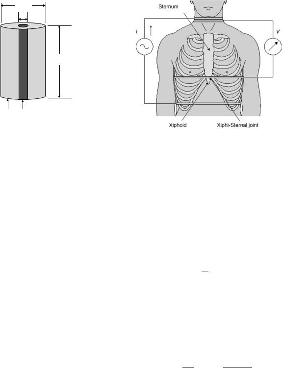
The Cylindrical Model. Many applications of bioimpedance measurement focus on primarily resistive changes. These techniques are all based on the cylindrical model (Fig. 2) represented by a tissue volume with uniform cross-sectional area (A), length (L), and resistivity (r) (14).

The resistance of the vessel segment is directly proportional to the resistivity of the conductive medium and length of the vessel segment and inversely proportional to the cross-sectional area of the vessel segment (Eq. 1). As shown in Fig. 2, as the cross-sectional area of the vessel segment increases from A1 to A3, the measured resistance decreases. Resistivity (r) is a tissue property that varies substantially between tissues. Typical tissue resistivities are shown in Table 1 (15).

Equation 1 can be modified to determine the volume of the tissue by multiplying both sides of the equation by L, substituting impedance (Z) for resistance, and solving for

A3

A2

A1

Figure 2. Cylindrical model of a vessel segment. A1–A3 represent cross-sectional area changes of the tissue of the interest (e.g., blood). Tissue length (L) is often determined by measurement electrode spacing. Blood resistivity (r) also determines the resistance (R) of the tissue volume. Resistance measured is directly proportional to the measured voltage and indirectly proportional to the constant alternating current (i) applied to the vessel segment.

The cylindrical model is based on several important assumptions: The electrical field, and hence current density, is homogeneous within the tissue of interest, the current is completely confined to the tissue of interest, and the values shown in Table 1 do not account for tissue anisotropy. Most biological tissues have lower resistivity in the longitudinal direction of cell or fiber orientation (12,16– 18). For example, the ratio of resistivity in the transverse to parallel direction can be > 3 in cardiac tissue (18). These assumptions may not be valid for some applications of bioimpedance such as the conductance catheter technique for chamber volume estimation (see below). Therefore, the

Table 1. Various Tissue Resistivities in ohms-meter (V m) (15)

200 BIOIMPEDANCE IN CARDIOVASCULAR MEDICINE

ATC

ABV

r TC

rBV L

CTC CBV

Figure 3. Parallel-column model of the thoracic cavity. This twocolumn model (CTC and CBV) represents a thoracic cavity segment of length (L), cross-sectional areas of the great blood vessels (ABV), and thoracic cavity segment (ATC), and resistivities of the thoracic cavity segment tissues (rTC) and blood volume (rBV).

cylindrical model must be adjusted for particular applications.

The Parallel-Column Model. The parallel-column model,

first described by Nyboer (5) (Fig. 3) is closely related to the cylindrical model, but accounts for current leakage into surrounding tissues. The model consists of a smaller cylindrical conductor (CBV) of length L representing the large blood vessels of the thoracic cavity (i.e., aortic and pulmonary arteries) embedded in a larger cylindrical conductor (CTC) of the same length (L) representing the tissues of the thoracic cavity. CBV consists of blood with specific resistivity (rBV) and time-varying cross-sectional area (ABV). CTC is assumed to be heterogeneous (i.e., bone, fat, muscle) with specific resistivity (rTC) and constant cross-sectional area (ATC). Thus, the cylindrical model of the time-varying volume can be modified:

where VT(t) represents the total volume change. As the distribution of the measured resistance and the net resistivity of the parallel tissues are unknown, calculation of absolute volume can be problematic. However, the constant volume term drops out when the change in volume is calculated from Eq. 3:

where Z0 is the basal impedance measured and DZ(t) is the pulsatile thoracic impedance change. Thus, Eq. 4 links the parallel cylindrical model to TEB estimates of stroke volume (DVBV).

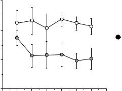
Noninvasive Measurement of Cardiac Output. Transthoracic electrical bioimpedance (TEB) was first intro-

Figure 4. Transthoracic band electrode placement for stroke volume estimates. The two outer-band electrodes supply the stimulus current (I ); the two inner electrodes measure the corresponding voltage (V ). Impedance is calculated from the ratio of V/I (15).

duced by Patterson et al. in 1964 (19). As shown in Fig. 4 (13), this system employs two pairs of band electrodes positioned at the superior and inferior ends of the thorax in the cervical and substernal regions, respectively. The outer electrode pair drives a constant current (I) and the inner electrode pair is used to measure the corresponding voltage (V), which is a function of the varying impedance changes during respiration and the cardiac cycle.

Noninvasive measurements of stroke volume can be determined with the configuration in Fig. 4 by applying Eq. 5.

"! #

Cardiac output may then be determined by multiplying stroke volume (SV) by heart rate (HR). DZ(t) is the measured time-varying impedance signal, and Z0 represents the nonpulsatile basal impedance.

Sramek et al. (20) modified Patterson et al.’s (19) parallel cylinder model into a truncated cone in order to improve stroke volume predictions (Eq. 6). The physical volume of the truncated cone was determined to be onethird the volume of the larger thoracic cylinder model.

Sramek et al. (20) also found that in a large normal adult population, the measured linear distance (L) is equal to 17% of body height (cm). Cardiac output is directly proportional to body weight (21). As ideal body weight is a linear function of overall height (22), the proportionality of height (H) to cardiac output can be represented in the first term of Eq. 6 by (0.17H)3/4.2.

Other empirical modifications to the original model have also been proposed in order to improve CO and SV estimates (20,22–28). In addition, various modifications to the external lead configuration have also been proposed to improve SV estimates, including the application of tranesophageal electrodes (29,30).

Several commercial bioimpedance systems are available for clinical noninvasive estimation of cardiac output and other hemodynamic parameters. The advantages of such systems include noninvasive application, relatively low cost, and lack of noninvasive alternatives. However, these techniques have gained somewhat limited clinical acceptance due to suspect reliability over a wide range of clinical conditions.

A myriad of validation studies of TEB estimates of cardiac output have been published with equivocal results (6,7,19,24,28,31–40). For example, Engoren et al. (35) recently compared cardiac output as determined by bioimpedance, thermodilution, and the Fick method and showed that the three methods were not interchangeable in a heterogenous population of critically ill patients. Their data showed that measurements of cardiac output by thermodilution were significantly greater than by bioimpedance. However, the bioimpedance estimates varied less than the thermodilution estimates for each subject. In contrast, a meta-analysis of impedance cardiography validation trials by Raaijmakers et al. (38) showed an overall correlation between cardiac output measurements using transthoracic electrical bioimpedance cardiography and a reference method of 0.82 (95% CI: 0.80–0.84). The performance of impedance measurement of cardiac output was similar in various groups of patients with different diseases with the exception of cardiac patients, in which group the correlation was decreased. Additional investigations by Kim et al. (41) and Wang et al. (42) used a detailed 3D finite element model of the human thorax to determine the origin of the transthoracic bioimpedance signal. Contrary to the theory that lead to the parallel column model formulae, these investigators determined that the measured impedance signal was determined by multiple tissues and

other factors that make reliable estimates of cardiac output over a wide variety of physiological conditions difficult. Nevertheless, commercially available impedance plethysmographs provide estimates of cardiac output that may be useful for assessing relative changes in cardiac function during acute interventions, such as optimization of implantable pacemaker programmable options such as AV delay (11).

Cardiac Cycle Event Detection. TEB also focuses on measurements of the change in impedance (DZ) and the impedance first time derivative (dZ/dt) measured simultaneously with the electrocardiogram (ECG). Figure 5 depicts a typical waveform of the aforementioned parameters. Note that the impedance change (DZ) and the impedance first time derivative (dZ/dt) are inverted by convention (43). The value of dZ/dt is measured from zero to the most negative point on the waveform. The ejection time (LVET) is an important parameter in determining stroke volume (Eqs. 5 and 6). This systolic time interval allows an estimation of cardiac contractility. The Heather Index (HI) is another proposed index of contractility from systolic time intervals determined by the dZ/dt waveform (33,44) (Eq. 7):

HI ¼ dZ=dtmax

QZ1

where dZ/dtmax (point C) is the maximum deflection of the initial waveform derived from the DZ waveform and QZ1 is the time from the beginning of the Q wave to peak dZ/dtmax (Fig. 5). In this figure, point Q represents the time between the end of the ECG p-wave (atrial contraction) and the beginning of the QRS wave (ventricular depolarization) (45). Point B depicts the opening of the aortic and pulmonic valves. After the ventricles depolarize and eject the blood volume into the aortic and pulmonary arteries, points X and Y represent the end systolic component of the cardiac cycle as closure of the aortic and pulmonic valves, respectively.

Passive mitral valve opening and passive ventricular filling begins at point O. Although the timing of the various

202 BIOIMPEDANCE IN CARDIOVASCULAR MEDICINE

fiducial notches of the dZ/dt waveform is well known, controversy remains with the origins of the main deflections and are not well understood (15).

Signal Noise. In TEB measurements, several filtering techniques have been proposed to attenuate undesired noise sources depending on which component of the impedance waveform is desired (i.e., respiratory, cardiac, or mean impedance) (47). Most of the signal processing techniques for impedance waves use ensemble averaging for the elimination of motion artifacts (48). A recent signal processing technique described by Wang et al. (48) uses the time-frequency distribution to identify fiducial points on the dZ/dt signal for the computation of left ventricular ejection time and dZ/dtmax. As shown in Fig. 5, many of the fiducial points on the dZ/dt waveform are clearly identifiable, but may be somewhat more difficult to observe under severe interference conditions.

Filtering techniques have also been proposed to eliminate noise caused by respiration such as narrow band-pass filtering around the cardiogenic frequency. However, such filtering techniques often eliminate the high frequency components of the cardiac signal and introduce phase distortion (49). To help alleviate this problem, various techniques to identify breathing artifacts with forward and backward filtering have been employed (50,51). Despite these techniques, motion artifact remains with unknown frequency spectra that may overlap the desired impedance frequency spectra during data acquisition. Adaptive filters represent another approach and may eliminate the motion artifact by tracking the dynamic variations and reduce noise uncorrelated to the desired impedance signal (49). Raza et al. (51) developed a method to filter respiration and low frequency movement artifacts from the cardiogenic electrical impedance signal. Based on this technique, the best range for the cutoff frequency appears to be from 30–50% of the heart rate under supine, sitting, and moderate exercise conditions (51).

Applications of Transthoracic Bioimpedance. Hypertension. TEB has emerged as a noninvasive tool to assess hemodynamic parameters, especially within the frame-

work of hypertension monitoring (24–28,52–54). Measurement of the various hemodynamic components such as stroke volume, ejection time, systemic vascular resistance, aortic blood velocity, thoracic fluid content, and contractility (i.e., Heather Index) using impedance cardiography in patients with hypertension allows more complete characterization of the condition, a greater ability to identify those at highest risk, and allows more effectively targeted drug management (25,53). Several studies have used TEB to evaluate hemodynamic parameters and demonstrated that TEB-guided therapy improves blood pressure control (53,55,56). For example, in a three month clinical study by Taler et al. (55) 104 hypertensive patients were randomized to either TEB-guided therapy or standard therapy. The results showed improved blood pressure control in the TEB-guided group. The investigators concluded that measurement of hemodynamic parameters with TEB methods was more effective than clinical judgment alone in guiding selection of antihypertensive therapies in patients resistant to empiric therapy (53).

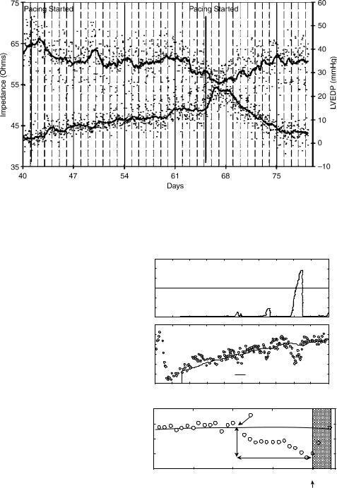
Pacemaker Programming. TEB estimates of cardiac index technique has been investigated as a noninvasive method to optimize AV delay intervals in pacemaker patients in an open-loop fashion (57,58). Ovsyshcher et al. (58) measured stroke volume changes at various programmed AV delays via impedance cardiography in dualchamber pacemaker patients. The optimal and worst programmed AV delays were identified as the settings that produced the highest and lowest cardiac index, respectively. As shown in Fig. 6 (58), the highest cardiac index values resulted with mean AV delays <200 ms and the lowest cardiac index values resulted with mean AV delays >200 ms.

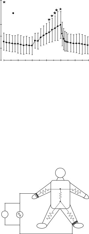
More recently, a study by Tse et al. (59) evaluated AV delay interval optimization during permanent left ventricular pacing using transthoracic impedance cardiography in conjuction with Doppler echocardiography over a range of AV intervals. This study revealed no significant difference between the optimal mean AV delay interval determined by transthoracic impedance cardiography and that determined by Doppler echocardiography. However, as shown in Fig. 7, the mean cardiac output at different AV

Figure 6. Highest and lowest cardiac indices at varied AV delays and pacing rates. Highest cardiac index values (closed circles) resulted with mean AV delays <200 ms and the lowest cardiac index values (open circles) resulted with mean AV delays >200 ms (58).

AV delay (ms)

300

200

Highest cardiac index

Lowest cardiac index

100

Heart rate

AV Interval (ms)

Figure 7. Cardiac output measured by impedance cardiography and Doppler echocardiography at various AV delay intervals (59).

delay intervals was significantly higher when measured by transthoracic impedance cardiography than when measured by Doppler echocardiography.

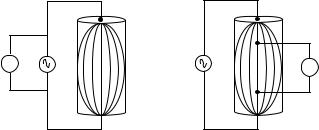
Electrical Impedance Tomography. Electrical impedance tomography (EIT) is a technique to reconstruct low resolution cross-sectional images of the body based on differential tissue resistivity (60). The image is created using an array of 16–32 electrodes, usually positioned around the thorax (Fig. 8). Impedance is computed from all electrodes as the drive electrodes rotate sequentially about the tissue surface. The ‘‘image’’ is then reconstructed using standard tomographic techniques. The advantages of EIT include low cost and the potential for ambulatory applications. The disadvantages include the low resolution of the image, the contribution of ‘‘out-of-plane’’ tissues to the ‘‘in-plane’’ image, and the limited clinical applications.

Recent improvements in hardware and software systems that increase the accuracy and speed of regional lung volume change have maintained interest in this technology (60–62). Besides pulmomary monitoring, other potential applications of EIT include neurophysiology, stroke detection, breast cancer detection, gastric emptying, and cryosurgery (63–66).

Lead Field Theory. An analysis of sensitivity is crucial to interpretation and application of EIT images as well as other bioimpedance applications. The sensitivity distribution of an impedance measurement provides the relation

Figure 9. High resolution computer simulated model of the thorax. Regions of both positive and negative sensitivity contribute to the total impedance measured. Negative impedance sensitivity regions, (1.54 V) and positive impedance sensitivity regions (red, 2.92 V) both contribute to the measure total impedance of 1.38 V. RL ¼ contribution of right lung to measured impedance. LR ¼ concontribution of left lung to measured impedance (62).

between the measured impedance resulting from the conductivity distribution of the measured region. It describes the relative contribution of each region to the measured impedance signal. The contribution of any region to the measurement is not always intuitively obvious and the magnitude of the sensitivity may be less than zero (Fig. 9). Therefore, the relative contribution of various tissues to the reconstructed ‘‘image’’ can be difficult to interpret.

The applicability of lead field theory in impedance measurements has been shown theoretically by Geselowitz (67). According to that theory, appropriate selection of the electrode configuration enables increased measurement sensitivity and selectivity to particular regions (68). Also, the measured impedance change (DZ) can be evaluated from the change in conductivity within a volume conductor Ds and the sensitivity distribution S by (67):

I

~

Current injection

Voltage measurement

V

V

V

Figure 8. Left: Cartoon representation of a system to generate an electrical impedance tomographic image: 16 electrodes around the chest inject currents and record the resultant voltage in a sequential manner. Right: Electrical impedance tomographic image of the thoracic cavity. Heart and lung tissue are distinguishable (60).

204 BIOIMPEDANCE IN CARDIOVASCULAR MEDICINE

10

8

6

4

2

0

The measurement sensitivity S is obtained by first determining the current fields generated by a unit current applied to the current injection electrodes and the voltage measurement electrodes. These two lead fields form the combined sensitivity field of the impedance measurement associated with the electrode configuration by:

where:

S ¼ the scalar field giving the sensitivity to conductivity changes at each location,

JLI ¼ the lead field produced by current excitation electrodes,

JLE ¼ the lead field produced by voltage measurement leads.

Therefore, sensitivity at each location depends on the angle and magnitude of the two fields and can be positive, negative, or null. The relative magnitude of the sensitivity field in a tissue segment provides a measure of how conductivity variation in that tissue segment will affect the detected DZ (69).

Lead field theory suggests that the relative contribution of a tissue to the measured impedance depends on the properties of the tissue, the symmetric arrangement of the tissues, and the geometry of the applied current and voltage electrodes. The precise relative contribution of various tissues to measure impedance is therefore difficult to predict (Fig. 10) (68).

Intrathoracic Bioimpedance

Minute Ventilation. As described earlier, respiratory rate can be estimated with TEB. However, intrathoracic impedance sensing has also been applied to measure respiratory rate and minute ventilation in implantable devices such as pacemakers and implantable cardiac defibrillators (ICDs). Intrathoracic impedance vector configurations typically consist of a tripolar arrangement with

bipolar pacing or ICD leads placed in the right ventricle (RV) and the device ‘‘can’’ (metal case or housing) placed subcutaneously in the left or right pectoral region. A variety of anode/cathode electrode arrangements are possible with current source electrodes such as the proximal electrode (RV-ring) to can or the distal electrode (RV-tip) to can and voltage sense electrodes between RV-coil to can. Typically, a low energy pulse of low current amplitude (1 mA with pulse duration of 15 ms) is delivered every 50 milliseconds (10). Figure 11 depicts a typical lead arrangement used for intrathoracic impedance measurements.

The electric fields generated with this electrode configuration must be arranged to intersect in parallel in order to provide the greatest sensitivity. The sensitivity of an electrode is proportional to the current density of the applied stimulus. Moreover, the sensitivity is highest close to the current-injecting electrodes and lowest toward the center of the tissue medium within the lead field vector,

Figure 11. Lead configuration for intracardiac impedance measurments. Stimulus current injected from RV-tip to can. Voltage is measured from RV-Ring to can. The large size of the can reduces electrode polarization effects of the tripolar lead configuration.

because the applied field current density is lowest in this region.

Experimental evidence indicates that the frequency and amplitude of the respiratory component of the bioimpedance signal are related to changes in both the respiratory rate and the tidal volume and, hence, the minute ventilation (MV). MV sensing in rate-adaptive pacing systems has also been shown to closely correlate with carbon dioxide production (VCO2) (10). This relationship has been applied in some commercially available pacemakers with automatic rate-adaptive pacing features (9,10).

As shown in Fig. 12 (46), the amplitude of impedance changes during respiration are significantly larger than the higher frequency cardiac components. By magnitude, the change in the cardiac component of the impedance waveform is in the range of 0.1–0.2 V, which correlates to approximately 0.3–0.5% of the thoracic impedance (DZ) (46). Moreover, each component has a different frequency, typically 1.0–3.0 Hz for cardiac activity and 0.1–1.0 Hz for respiratory activity (9). This differentiation allows extraction of each signal by specific filtering techniques.

In general, the minute-ventilation sensor is characterized by a highly proportional relationship to metabolic demand over a wide variety of exercise types (10). However, optimal performance of impedance-based MV sensors to control pacing rate during exercise often requires careful patient-specific programming.

Fluid Status. Fluid congestion in the pulmonary circulation due to volume overload results in preferential transport of fluid primarily into the extracelluar fluid space and not into the intracellular compartments. Clinical symptoms to assess fluid overload include hypertension, increased weight, pulmonary or peripheral edema, dyspnea, and left ventricular dysfunction. Recently, implantable device-based bioimpedance measurements have been applied to detect thoracic fluid accumulation in patients with congestive heart failure (CHF) and to

Figure 12. Respiratory variation in impedance waveform. Electrocardiogram (ECG) shown with DZ waveform. DZ waveform is comprised of higher frequency cardiac components superimposed on the lower frequency respiratory variation component (46).

provide early warning of decompensation caused by factors such as volume overload and pulmonary congestion (32,70,71). This application is the result of a substantial body of new and historical experimental evidence (32,70–73).

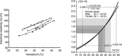
Externally measured transthoracic impedance techniques have been shown to reflect alterations in intrathoracic fluid and pulmonary edema in acute animal and human studies (72). The electrical conductivity and the value for transthoracic impedance are determined at any point in time by relative amounts of air and fluid within the thoracic cavity (73). Additional studies have suggested that transthoracic impedance techniques provide an index of the fluid volume in the thorax (32,71). Wang et al. (70) employed a pacing-induced heart failure model to demonstrate that measurement of chronic impedance using an implantable device effectively revealed changes in left ventricular end-diastolic pressure in dogs with pacinginduced cardiomyopathy (Fig. 13) (70). Several factors were identified that may influence intrathoracic impedance with an implantable system, including (1) fluid accumulation in the lungs due to pulmonary vascular congestion, pulmonary interstitial congestion, and pulmonary edema; (2) as heart failure worsens, heart chamber dilation and venous congestion occur and pleural effusion may develop; and (3) after implant, the tissues near the pacemaker pocket swell and surgical trauma can cause fluid buildup (70).

Yu et al. (74) also showed that sudden changes in thoracic impedance predicted eminent hospitalization in 33 patients with severe congestive heart failure (NYHA Class III–IV). During a mean follow-up of 20.7 8.4 months, 10 patients had a total of 25 hospitalizations for worsening heart failure. Measured impedance gradually decreased before admission by an average of 12.3 5.3% (p < 0.001) over a mean duration of 18.3 10.1 days. The decline in impedance also preceded the symptom onset by a mean lead time of 15.3 10.6 days (p < 0.001). During hospitalization, impedance was inversely correlated with

206 BIOIMPEDANCE IN CARDIOVASCULAR MEDICINE

Figure 13. Impedance vs. LVEDP during pacing-induced heart failure. Intrathorcic impedance via an implantable device-lead configuration and LVEDP are inversely correlated in a canine model of pacing-induced cardiomyopathy. A general trend for impedance to decrease as heart failure developed is shown. Once pacing induced heart failure was terminated, LVEDP and impedance returned to basal levels (70).

pulmonary wedge pressure (PWP) and volume status with r ¼ 0.61 (p < 0.001) and r ¼ 0.70 (p < 0.001), respectively. Automated detection of impedance decreases was 76.9% sensitive in detecting hospitalization for fluid overload with 1.5 false-positive (threshold crossing without hospitalization) detections per patient-year of followup. Thus, intrathoracic impedance from the implanted device correlated well with PWP and fluid status, and may predict eminent hospitalization with a high sensitivity and low false-alarm rate in patients with severe heart failure (Fig. 14) (74). Some commercially available implantable devices for the treatment of CHF or ventricular tachyarrhythmias now continually monitor intrathoracic impedance and display fluid status trends. This information is then provided to the clinician via direct-device interrogation or by remote telemetry.

Volume Conductance Catheter. The conductance catheter technique, first described by Baan et al. (8), enables continuous measurements of chamber volume, particularly left ventricular (LV) volume. This method has been used extensively to assess global systolic and diastolic ventricular function (75). In many respects, the conductance catheter revolutionized the study of cardiovascular mechanics in both the laboratory and clinical settings by making the study of ventricular pressure-volume relationships practical. The technique led to a renaissance of cardiac physiology over the past 25 years (76) by increasing the understanding of the effect of pharmacologic agents, disease states, pacing therapies, and other interventions on cardiovascular function. Conductance catheter systems are available for clinical and laboratory monitoring applications, including a miniature system capable of measuring LV volume and pressure in mice (77).

The conductance methodology is based on the parallel cylinder model (Fig. 3). However, the cylindrical model assumes that the volume of interest has a uniform crosssectional area across its length. Therefore, the ventricular volume is subdivided into multiple segments determined by equipotential surfaces bounded by multiple sensing electrodes along the axis of the conductance catheter (Fig. 15).

Figure 14. Fluid status monitoring with an implanted device. A: Operation of algorithm for detecting decreases in impedance over time. Differences between measured impedance (bottom; 8) and reference impedance (solid line) are accumulated over time to produce fluid index (top). Threshold values are applied to fluid index to detect sustained decreases in impedance, which may be indicative of acutely worsening thoracic congestion. B: Example of impedance reduction before heart failure hospitalization (arrow) for fluid overload and impedance increase during intensive diuresis during hospitalization. Label indicates reference baseline (initial reference impedance value when daily impedance value consistently falls below reference impedance line before hospital admission). Magnitude and duration of impedance reduction are also shown. Days in hospital are shaded (74).

Figure 15. Conductance catheter modeled in the left ventricle (LV). Stimulus current is injected from the proximal and distal catheter electrodes. Voltage is measured between the remaining adjacent electrode pairs. Total conductance is calculated by the summation of all segmental conductances measured in the individual segments.

The two most distal electrodes are used to generate an electric field, typically 0.4 mA p-p, at 20 kHz. The remaining electrodes are used in pairs to measure the conductance of several segments (n ¼ number of segments), which represent the instantaneous volumes of the corresponding segment. The conductance is then converted to volume by modifying Eq. 2:

n

VðtÞ ¼ rL2 S GiðtÞ ð10Þ

i¼1

where G is the time-varying conductance of segment i. However, the conductance technique also violates two other key assumptions of the cylindrical model. First, the electrical field generated by the drive current electrodes is not homogenous and, second, the electric field is not confined to the chamber of interest (i.e., the LV). Thus, the multiple segment cylindrical model has been modified in order to allow conductance catheter estimates of volume to agree with gold standard estimates such as echocardiography (Eq. 11):

where correction factor a accounts for nonhomogeneity of the electric field and the correction factor VP accounts for the current leakage into the surrounding tissues. The terms a and Vp are related and may vary somewhat during the cardiac cycle (16,78). Various methods have been applied to determine the values of a and VP, including the method of hypertonic saline injection.

Recently, the concept of dual-frequency excitation has been applied to estimate VP for conductance volume measurements in mice (79). This method takes advantage of the relative reactive components of impedance between blood and tissue (80). Despite some theoretical limitations regarding the basic assumptions of field heterogeneity and current leakage, the conductance catheter technique has also been applied to the study of biomechanics in other chambers besides the left ventricle, including the right ventricle (81), right and left atria (82), and aorta (83,84).

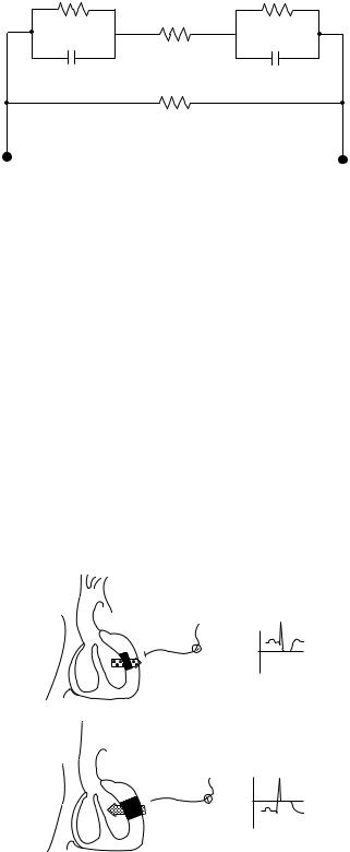
Other Pacing Applications. Intracardiac impedance, or transvalvular impedance (TVI), can be used in the assessment of cardiac hemodynamics. This method involves determining the impedance between pacemaker leads in the right atrium and ventricle using a typical dual-cham- ber pacing configuration. The TVI waveform can be categorized into atrial, valvular, and ventricular components (Fig. 16) (85). Information derived from the atrial component may be useful to identify the loss of electrical capture in the atrium, or the impairment in atrial hemodynamic function associated with supraventricular tachyarrhythmias. The valvular and ventricular components may provide information on the presence, timing, and strength of ventricular mechanical activity (86).

In a study performed by Gasparini et al. (85), the representative TVI tracings (Fig. 16) were recorded from atrial ring to ventricular tip. TVI was measured by application of 64 Hz subthreshold current pulses of 125 ms duration and the amplitude ranging from 15 to 45 mA. The TVI

Figure 16. TVI during spontaneous A-V sequential activity. Fiducial points on the TVI waveform used to optimize A-V delay. t1 corresponds to the end of atrial systole; t2 corresponds to the end of ventricular ejection (85).

208 BIOIMPEDANCE IN CARDIOVASCULAR MEDICINE

signal was recorded without high-pass filtering to determine the absolute minimum and maximum impedance in each cardiac cycle, which were assumed to reflect the enddiastolic volume and the end-systolic volume, respectively. TVI may represent a useful approach to determine hemodynamic parameters such as stroke volume, ejection fraction, pre-ejection interval, and atrio-ventricular delay. One significant advantage with this technique is that the source and sense leads are of those typically used in pacing systems and offer the advantage of a high signal-to-noise ratio (86). Moreover, the use of this technique has the potential to differentiate atrial from ventricular function that would be paramount if this technique is used for atrioventricular delay optimization (87).

Hematocrit Measurement. Measurement of the resistivity of whole blood has been investigated by a number of researchers, particularly in the area of transthoracic impedance techniques (88–91). A number of investigators have found blood resistivity to be an exponential function of hematocrit (Fig. 17) (15,89–95). These studies have demonstrated a strong correlation between the electrical resistivity of blood at frequencies between 20 to 50 kHz, as the red blood cell is the major resistive component in blood, compared with the relatively conductive plasma. Pop et al. (93) employed a four ring catheter electrode system with narrow electrodes spacing (2 mm center-to-center) to estimate hematocrit in the right atrium of anesthetized pigs. As shown in Fig. 17, good correlation existed between the hematocrit of blood and its electrical resistivity (r2 ¼ 0.95–0.99). Moreover, this study also showed a strong correlation between whole blood viscosity and electrical resistivity.

This interesting observation implies that intracardiac impedance has potential to monitor thrombosis risk in patients with hyperviscosity.

Blood Flow Conductivity Based on Erythrocyte Orientation. The electrical properties of blood are of practical interest in medicine because blood has the highest conductivity of all living tissues (89,96,97). Blood is a heterogeneous suspension of erthrocyctes that have a higher resistivity than the suspending fluid (plasma). The resistivity of blood is a function of the resistivities of plasma,

the (fractional) packed-cell volume or hematocrit, and the orientation of the erythrocytes, due to their biconcave shape (98). The orientation of the erythrocytes can be influenced by the viscous forces in flowing blood, resulting in a shear rate-dependent resistivity. In stationary blood, the erythrocytes assume a random distribution while in flowing blood, the plane of the erythrocytes becomes oriented parallel to the axis of flow (99). Thus, minimum resistance occurs when the erythrocytes are oriented in an axial direction, parallel to the stream line. Conversely, maximum resistance occurs when the erythrocytes are oriented in a transverse direction to the stream line (100). The electrical properties of pulsatile blood flow are important when applying transthoracic bioimpedance to estimate cardiac output. In an experiment performed by Katsuyuki et al. (101), erythrocyte orientation, deformation, and axial accumulation caused differences in resistance between flowing and resting blood. Frequency characteristics of blood resistance under pulsatile flow showed that at low pulse rates, the resistance change was minimal, whereas at higher pulse rates, the resistance change increased because the orientation of the erythrocytes cannot follow the rapid changes of pulsatile blood flow. These results suggest that one mechanism of the varying resistance of blood in the aorta during pulsatile blood flow occurs because the orientation of the erythrocyte changes due to shear as a function of heart rate. Therefore, hemodynamic parameters such as cardiac output measured by impedance plethysmography must take into account the anisotropic electrical properties of oriented erythrocytes in blood. Moreover, the resulting resistance of flowing blood depends on the direction of the electrical field applied for impedance measurement and may be affected by the orientation of the erythrocytes during pulsatile flow (101).

REACTIVE APPLICATIONS OF BIOIMPEDANCE

Tissue Impedance

The reactive component of tissue impedance does not contribute significantly to measured impedance when the driving frequency range is less than 1 kHz (8,15). However,

I

V

∆t

Figure 18. Relationship in phase angle and amplitude for tissue electrical properties. This example shows a capacitive tissue segment since the current waveform (I) leads the voltage waveform (V ) by phase angle (u) (103).

at higher driving current frequencies, the reactive component may contribute more substantially. As different tissues have different reactance, different frequencies may be selected for impedance measurement in order to discriminate various tissues (15,102).

Tissue impedance is characterized by four components: the in-phase component of voltage (V) with respect to the current intensity (I), the tissue resistance (R), and the phase angle (u). The phase angle represents the time delay between the voltage and current intensity waves due to the capacitance of cell membranes (Fig. 18) (103).

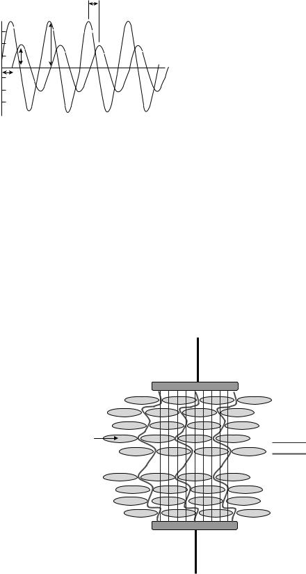
Figure 19 shows cellular tissue structure representing alternating current distribution between a bipolar elec-

trode pair at high and low frequencies. The change in polarity that occurs with AC current causes the cell membrane to charge and discharge at the rate of the applied frequency, and the impedance decreases as a function of increased frequency, because the amount of conducting volume increases through intracellular space. At higher frequencies, the rate of cell membrane charge and discharge becomes such that the effect of the cellular membrane on measured impedance becomes insignificant and the current flows through the intracellular and extracellular space (104).

Capacitance causes the voltage to lag behind the current (Fig. 18), creating a phase shift that is quantified as the angular transformation (u) of the ratio of reactance to resistance (105). Note that the uniform orientation of cells in a tissue (Fig. 19) can result in anisotropy of electrical properties. That is, impedance will be lower in the longitudinal versus transverse direction of the tissue segment cellular structure (12,18).

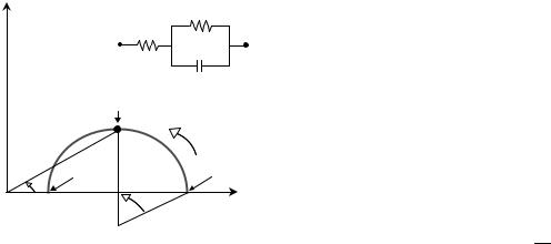
The parallel-column model (Fig. 3) must be modified to describe higher frequency applications of bioimpedance in which the capacitive properties of the cell membranes become important. The Cole–Cole plot (Fig. 20) is a useful characterization of the three element RC model that describes the behavior of tissue impedance as a function of frequency (f), impedance (Z), resistance (R), reactance (XC), and phase angle (f) (103). The real components (R1 and R2) can be plotted versus the negative imaginary component of the capacitor (C) with reactance (XC) in the complex series impedance (R þ jXC), with the frequency as a parameter where j ¼ ðp 1Þ (15). As the frequency is

210 BIOIMPEDANCE IN CARDIOVASCULAR MEDICINE

Figure 20. Cole–Cole plot and equivalent tissue impedance circuit. Resistance (abscissa) and reactance (ordinate) plotted as a function of frequency. A three-element electrical equivalent tissue impedance model is shown. At low frequency (fL), the equivalent circuit is resistive and R0 ¼ R1 þ R2. As the frequency increases, the phase angle (f) increases until the resistance and reactance are equal at the characteristic frequency of the tissue (fC). As the frequency increases beyond the characteristic frequency, the reactive element C is reduced to a low impedance and the tissue displays purely resistive properties where R1 ¼ R1. The depressed locus at angle a is presumed to represent electrode polarization.

changed between R0 and R1, the impedance will change continually along a curve in the R-X plane. At very low frequencies (fL), the capacitive component of the system is effectively an open circuit so the reactance is equal to zero and the measured impedance (Z) is purely resistive (R0). As the frequency increases, reactance (XC) increases in proportion to resistance causing the phase angle (f) to increase until a maximum angle is reached at the critical (characteristic) frequency (fC). As shown in Fig. 20, phase angle is positively associated with reactance and negatively associated with resistance (106). Beyond the critical frequency, the reactance begins to decrease in proportion to resistance with increasing frequency and, at very high frequencies (fH), the capacitive component is essentially short-circuited so the measured impedance is purely resistive at R1 (105).

If impedance of a tissue is measure over a broad spectrum, then the resultant impedance Cole–Cole plot can be fit to the three element model or other similar lumpedparameter models. Changes in the model elements can reflect changes in tissue properties due to pathological conditions such as ischemia (see below). In many biologic systems, the center of loci of the plot lies below the real axis and is represented by the angle a, a fixed number between 0 and 1 (2). This behavior can only be modeled by adding an inductive element to the electrical parameter model shown in Fig. 20. However, the physiological interpretation of the inductance is uncertain. Fricke et al. hypothesized that a possible source of this observed inductance might be electrode polarization (107). These investigations demonstrated behavior similar to constant depression angle of electrode polarization. They demonstrated that a frequency-dependent resistance and reactance could mathematically assume a constant depression angle (2). However, the physiologic explanation for a > zero remains

controversial. An additional theory related to the origin of the depressed loci is the distribution of time constants in a heterogeneous tissue segment. This distribution could result from variability in cell size or variability in properties of the individual cells (2).

Ischemia Detection. Tissue degradation due to ischemia can alter both the real and reactive components of bioimpedance (40). The dielectric polarization of matter (e.g., myocardial tissue) is given by the dimensionless parameter e0, which is called dielectric permittivity. e0 describes the capacitance increase of a capacitor filled with matter:

where:

C ¼ a capacitor with matter (i.e., cellular structure), C0 ¼ vacuum capacitor.

As the dielectric polarization processes are frequencydependent, they show relaxation phenomena with increasing frequency (108). The relaxation process is defined by the complex dielectric permittivity e, thus:

where:

e0 ¼ dielectric permittivity, e00 ¼ dielectric loss factor, v ¼ 2pf,

f ¼ frequency of stimulus current, i ¼ imaginary unit ðp 1Þ.

The method of dielectric spectroscopy has been proposed to investigate heart tissue during global ischemia, because the dielectric polarization of matter can be measured by the application of weak electric fields. An electrical circuit model to describe myocardial ischemia, initially developed by Gersing (109) and modified by Schaefer et al. (108), is depicted in Fig. 21. This model can be considered as a variation of the simplified three element physiologic model as shown in Fig. 20. The resistance Rext describes the properties of the extracellular electrolyte, and the resistance Rint describes the intracellular cytosol. This model assumes that the transcellular current has to pass the membrane with capacitance Cm and the resistance Rm, through the cytosol, and from cell to cell through the interstitial membranes described by Cis or, alternatively, through gap junctions with resistance Rg (108,109). Application of this model enables quantification of the variation of intracellular coupling via gap junctions due to myocardial ischemia (108–111).

The measurement of alterations in impedance spectra with ischemia is often referred to as impedance spectroscopy. Myocardial electrical impedance (MEI), a specific application of impedance spectroscopy, has been shown to

Figure 21. Electronic equivalent model of heart tissue. Electrical elements consist of the intracellular (Rint) and extracellular resistance (Rext), cellular membrance capacitance (Cm) and resistance (Rm), cell-to-cell interstitial membrane capacitance (Cis), and gap junction resistance (Rg).

identify localized and global myocardial tissue in various disease states in in vitro and in vivo experimental models (112).

Recently, MEI has been used in conjunction with electrocardiogram (ECG) ST-segment deviations to assess the magnitude of the ischemic region of the myocardium (103,112–116).

Injury currents, secondary to myocardial ischemia result in ST-segment displacements in the ECG of patients with myocardial ischemia (117). Injury currents deriving from resting depolarization in ischemic myocardial cells are associated with slow conduction through the myocardium. The mechanisms by which these injury currents correlate with the impedance spectroscopy alterations in the ischemic myocardial tissue are well described (103,108,109,112–117). Figure 22 depicts a segment of

Figure 22. Ischemic regions of myocardial tissue and corresponding ST-segment. Subendocardial ischemia (top) with depressed ST-segment. Transmural ischemia (bottom) with elevated STsegment (117).

the myocardium with subendocardial and transmural ischemic tissue. Blood flow through the heart is interrupted during ischemia, and the tissue undergoes progressive changes leading to irreversible loss of its viability (108). Transmural ischemia causes ST-segment elevation and subendocardial ischemia causes ST-segment depression (117). The electrocardiographic differences between transmural and subendocardial ischemia are clinically important. Supply ischemia, as occurs following total interruption of flow through a coronary artery supplying a large area of the left ventricle, typically causes ST-segment elevation (63). In contrast, demand ischemia, as occurs during a stress test, begins in the subendocardial regions of the left ventricle and causes ST-segment depression (117).

The mechanism by which MEI changes with ischemia is not certain, but may well be associated with ultrastructural changes or cellular biochemical changes that occur in the myocardial tissue similar to those viewed by STsegment deviations (113). The increase in MEI may result from reductions in the conductive fluid volume in the affected region of the myocardium (113). Gap junctions play a critical role in the propagation of electrical impulse in the heart, and its conductivity has been shown to be reduced and eventually abolished during ischemia and rapidly restored during reperfusion (103). Thus, gap junction closure is a reasonable hypothesis to explain observed impedance changes with ischemia. The intraischemic variation of intracellular and extracellular coupling is one possible explanation for the observed impedance changes of the dielectric frequency spectrum (108).

As MEI correlates with myocardial tissue viability (118,119), the measure has several important potential monitoring applications. Intraoperatively, MEI could be used to detect ischemia in aortic or myocardial tissue during cardiopulmonary bypass surgery as an early indication of damage. Following cardiopulmonary bypass, MEI could be used to assess reperfusion afforded by the new grafts. MEI could also aid in drug titration after cardiac surgery as well as to chronically monitor tissue perfusion with implantable devices such as pacemakers or cardio- verter-defibrillators, or with patients whom have received a heart transplant (12,113,120).

In a study performed by Howie et al. (113), acute ischemia was induced in anesthetized dogs via left anterior descending (LAD) coronary artery occlusion for randomly assigned periods of 15, 30, 45, 60, or 120 min. MEI was simultaneously recorded using ventricular pacing leads sutured into the exposed heart tissue. As shown in Fig. 23, MEI increased immediately after LAD coronary artery occlusion and returned to baseline following reperfusion. A statistically significant increase occurred from baseline impedance when compared at 64, 68, 72, 76, and 80 min (113). This intracardiac technique used by Howie et al. suggested other possible applications for MEI with implantable devices and intracardiac pacing/monitoring leads. However, further development in the direction of optimal electrode placement to isolate the targeted tissue region and obtain the highest quality data for diagnosis of tissue alteration is warranted (12).

212 BIOIMPEDANCE IN CARDIOVASCULAR MEDICINE

Myocardial impedance (Ω)

Figure 23. Change in myocardial impedance during LAD coronary artery occlusion (113).

1100

Significantly (P < 0.05) Greater than Baseline

900

800

700

600

Dialysis. Whole-body bioimpedance spectroscopy has been proposed by several investigators for measuring extracellular (ECW) and intracellular (ICW) water volumes in dialysis patients in order to assess nutritional status and to monitor hydration (121–125). An adequate assessment of body water compartments is crucial in dialysis patients because overhydration and underhydration are often difficult to detect and may result in severe morbidity in this population (126). Despite the continuous progress in the delivery of renal replacement therapy, mortality in patients on maintenance dialysis remains higher than in the general population (127).

During acute volume overload, most of the extra fluid collects in the ECW not the ICW. At very low frequencies, current only penetrates the ECW because the cell membrane acts as a capacitor and the impedance becomes equal to the ECW resistance (see Fig. 19). At very high frequencies, the injected current penetrates both the ECW and the ICW, and the impedance represents the total body water (TBW) resistance (125). Several investigators (128–131) have used singleand multiple-frequency impedance to monitor fluid shifts during hemodialysis. However, when attempting to determine precise fluid volumes from the measured impedance, difficulties occur due to the complex geometry of the human body and electrical inhomogeneity of nonconducting elements such as bone and fat (125). Signal processing methods to account for these aforementioned difficulties are described in the literature (104,124,125,132).

Whole-body bioelectrical impedance measurements typically apply single (e.g., 50 kHz) (133) or multifrequency (e.g., 5 to 1000 kHz) alternating currents applied via cutaneous electrodes placed on the hands and feet with more proximal electrodes uses for voltage measurements (126). The precise method for calculation of body fluid volumes depends on whether the single-frequency or multiple-fre- quency method is applied. The single-frequency method often uses an empirically derived regression formula to assess TBW, whereas the multiple-frequency method predicts the volume of TBW and ECW from a general mixture theory, assuming specific resistance values for ECW and

ICW (104,126,134). Moreover, the contribution of body weight, which is strongly related to ECW and TBW, is greater in the regression approach compared with the mixture approach (126).

Although reliable measurements of fluid content in dialysis patients have been reported (121–131), uncertainty remains regarding the agreement of whole-body bioimpedance in dialysis patients with tracer dilution techniques, which are considered the gold standard methods (126). One explanation for the lack of satisfactory agreement between techniques is that whole-body bioimpedance techniques consider the body as a multiple conductive cylinder model (e.g., arms, legs, trunk) connected in series (Fig. 24). With conductors connected in series, conductors with the smallest cross-sectional area (e.g., extremities) will determine most of the resistance, whereas the component with the largest cross-sectional area (e.g., trunk) will have minimal contribution to the resistance

Thoracic Cavity Conductance (1/RTC) þ Right Leg Conductance

(1/RRL).

although it contains a significant amount of body water (126). However, assessment of the sum of segmental bioelectrical impedance analysis measurements, which take into account resistance of the extremities and the trunk independently, have been shown to detect changes in trunk water more accurately (135). A seminal study performed by Patterson et al. (136) used multiple linear regression analysis combining data measured independently from the arms, legs, and trunk correlated with weight change on patients undergoing hemodialysis, gave a correlation coefficient of 0.87, whereas the correlation coefficient from measurements between just the wrist and ankle was 0.64.

Pulmonary Edema Detection. Patients developing pulmonary edema initially accumulate fluid in the interstitial spaces of the lung. As the condition progresses, fluid ultimately accumulates in the alveoli. To accurately measure pulmonary fluid status, the different bioelectric properties of blood, lung tissue, and extravascular fluid must be considered, and an impedance parameter not influenced by the patient’s geometry should be used (137). Thus, using a dual-frequency measurement of thoracic impedance, an impedance ratio can be calculated that represents the ratio between intracellular and extracellular water. This ratio, therefore, changes as a result of the fluid shift caused by edema formation. As the low frequency current only passes through the extracellular resistance, the measured low frequency impedance (ZLF) over a specified thoracic length equals the total extracellular resistance. As the frequency is increased, current is divided over the intracellular and extracellular compartments. Therefore, the measured high frequency impedance (ZHF) over a specified thoracic length equals the parallel equivalent of intracellular and extracelluar impedance. Thus, a dual-frequency impedance ratio that represents the intracellular/extracellular impedance fraction can be defined by ZHF/ZLF. As pulmonary fluid accumulates in the extracellular space, the impedance ratio increases (137).

BIBLIOGRAPHY

Cited References

1.Grimnes S, Martinsen O. Bioimpedance and Bioelectricity Basics. London: Academic Press; 2000. p 313–320.

2.Ackmann J, Seitz M. Methods of complex impedance measurements in biologic tissue. CRC Crit Rev Biomed Eng 11(4):281–311.

3.Schwan HP. The bioimpedance field: Some historical observations. Proceedings of the 4th International Conference on Electrical Bioimpedance. 1995; 1–4.

4.Nyboer J, et al. Radiocardiograms: Electrical impedance changes of the heart in relation to electrocardiograms and heart sounds. J Clin Invest 1940; 19:963.

5.Nyboer J. Electrical impedance plethysmography: A physical and physiologic approach to peripheral vascular study. Circulation 1950;2:811–821.

6.Kubicek W, et al. Development and evaluation of an impedance cardiac output system. Aerospace Med 1966;37:1208– 1212.

7.Djordjevich L, Sadove M. Basic principles of electrohemodynamics. J Biomed Eng 1981; 3:25–33.

8.Baan J, et al. Continuous measurement of left ventricular volume in animals and humans by conductance catheter. Circulation 1984;70(5):812–823.

9.Min M, Parve T, Kink A. Thoracic impedance as a basis for pacing control. Ann NY Acad Sci 1999;873: 155–166.

10. Ellenbogen K, Wood M. Cardiac Pacing and ICD’s. 3rd ed. Malden (MA): Blackwell Science; 2002. p 106– 109.

11.Kindermann M, et al. Optimizing the AV delay in DDD pacemaker patients with high degree AV block: Mitral valve doppler versus impedance cardiography. PACE 1997;20(10 pt 1):2453–2462.

12.Steendijk P, et al. The four-electrode resistivity technique in anisotropic media: Theoretical analysis and application on myocardial tissue in vivo. IEEE Trans Biomed Eng 1993;40(11):1138–1147.

13.Nyboer J. Electrorheometric properties of tissues and fluids. Ann NY Acad Sci 1970;170(2):410–420.

14.Geddes LA, Hoff HE. The measurement of physiological events by electrical impedance, a review. Am J Med Electron 1964; 14:16–27.

15.Malmivuo J, Plonsey R. Bioelectromagnetism. In: Principles and Application of Bioelectric and Biomagnetic Fields. United Kingdom: Oxford Univeristy Press; 1995. p 141, 405–419.

16.Hettrick DA, Battocletti JH, Ackmann JJ, Linehan JH, Warltier DC. Effects of physical parameters on the cylindrical model for conductance volume measurement. Ann Biomed Eng 1997;24:126–134.

17.Hettrick D, et al. Finite element model determination of correction factors used for measurement of aortic diameter via conductance. Ann Biomed Eng 1999;27(2): 151–159.

18.Roberts DE, Hersh LT, Scher AM. Influence of cardiac fiber orientation on wavefront voltage, conduction velocity, and tissue resistivity in the dog. Circ Res 1979; 44:701–712.

19.Patterson R, et al. Development of an electrical impedance plethysmography system to monitor cardiac output. Proceedings of the First Annual Rocky Mountain Bioengineering Symposium, 1964: 56–71.

20.Sramek B, Rose D, Miyamoto A. A stroke volume equation with a linear base impedance model and its accuracy, as compared to thermodilution and magnetic flowmeter techniques in humans and animals. Proceedings of the Sixth International Conference on Electrical Bioimpedance, Zadar, Yugoslavia, 1983: 38.

21.Milnor WR. Hemodyanmics. Baltimore: Williams & Wilkins Co.; 1982. p 155.

22.Statistical Bulletin. Metropolitan Life Foundation, JanuaryJune 1983. p 64.

23.Quail A, et al. Thoracic resistivity for stroke volume calculation by impedance cardiography. J Appl Physiol 1981;50:191.

24.Albert N, et al. Equivalence of bioimpedance and thermodilution in measuring cardiac output in hospitalized patients with advanced, decompensated chronic heart failure. Am J Crit Care 2004;13:469–479.

25.Van DeWater J, et al. Impedance cardiography: The next vital sign technology? Chest 2003;123: 2028–2033.

26.Drazner M, et al. Comparison of impedance cardiography with invasive hemodynamic measurments in patients with heart failure secondary to ischemic or nonischemic cardiomyopathy. Am J Cardiol 2002;89:993–995.

27.Sageman W, Riffenburgh R, Spiess B. Equivalence of bioimpedance and thermodilution in measuring cardiac index

214 BIOIMPEDANCE IN CARDIOVASCULAR MEDICINE

after cardiac surgery. J Cardiothroracic Vasc Anesth 2002; 16:8–14.

28.Yung G, et al. Comparison of impedance cardiography to direct Fick and thermodilution cardiac output determination in pulmonary arterial hypertension. Congest Heart Fail 2004;10(Suppl 2):7–10.

29.Patterson RP. Possible technique to measure ventricular volume using electrical impedance measurements with an oesophageal electrode. Med Biol Eng Comput 1987;25:677– 679.

30.Hettrick DA, et al. Correlation of esophageal conductance measurements with aortic and left ventricular diameters and stroke volume. IEEE Trans Biomed Eng 2000;47:559– 564.

31.Patterson R. Handbook of Biomedical Engineering. Bioelectric Impedance Measurements. Boca Raton, FL: CRC Press; 1995. p 1223–1230.

32.Ebert T, et al. The use of thoracic impedance for determining thoracic blood volume changes in man. Aviation Space Environ Med 1986 57:49–53.

33.Mancini R, et al. Cardiac output and contractility indices: Establishing a standard in response to low-to-moderate level exercise in healthy men. Arch Phys Med Rehabil 1979;60:567–573.

34.Levett J, Replogle R. Thermodilution cardiac output: A critical analysis and review of the literature. J Surg Res 1979;27:392–404.

35.Engoren M, Barbee D. Comparison of cardiac output determined by bioimpedance, thermodilution, and the Fick method. Am J Crit Care 2005;14(1):40–45.

36.Imhoff M, Lehner J, Lohlein D. Noninvasive whole-body electrical bioimpedance cardiac output and invasive thermodilution cardiac output in high-risk surgical patients. Crit Care Med 2000;28:2812–2818.

37.Cotter G, et al. Accurate, Noninvasive continuous monitoring of cardiac output by whole body electrical bioimpedance. Chest 2004;125:1431–1440.

38.Raaijmakers E, et al. A meta-analysis of published studies concerning the validity of thoracic impedance cardiography. Ann NY Acad Sci 1999;873: 121–134.

39.Patterson R, Witsoe D. Impedance stroke volume compared with dye and electromagnetic flowmeter values during drug induced inotropic and vascular changes in dogs. Ann NY Acad Sci 1999;873:143–148.

40.Min M, Ollmar S, Gersing E. Electrical impedance and cardiac monitoring: Technology, potential and applications. Int J Bioelectromag 2003;5(1):53–56.

41.Kim D, et al. Origins of the impedance change in impedance cardiography by a three-dimensional finite element model. IEEE Trans Biomed Eng 1988 ;35(12): 993– 1000.

42.Wang L, Patterson R. Multiple sources of the impedance

cardiogram based on 3-D finite difference human thorax models. IEEE Trans Biomed Eng 1995;42(4): 141–148.

43.Wang X, et al. An impedance cardiography system: A new design. Ann Biomed Eng 1989;17: 535–556.

44.Summers R, Kolb J, Woodward L. Differentiating systolic from diastolic heart failure using impedance cardiography. Academ Emerg Med 1999;6(7):693–699.

45.Lababidi Z, et al. The first derivative thoracic impedance cardiogram. Circulation 1970;41(4): 651–658.

46.Osypka M, Berstein D. Electrophysiologic principles and theory of stroke volume determination by thoracic electrical bioimpedance. Non-invasive monitoring using thoracic bioimpedance. AACN Clin Issues 1999;10(3): 385–399.

47.Christov I. Dynamic powerline interference subtraction from biosignals. J Med Eng Technol 2000;24(4):169– 172.

48.Wang X, Sun H, Van DeWater J. An advanced signal processing technique for impedance cardiography. IEEE Trans Biomed Eng 1995;42(2):224–230.

49.Barros A, Yoshizawa M, Yasuda Y. Filtering noncorrelated noise in impedance cardiography. IEEE Trans Biomed Eng 1995;42(3):324–327.

50.Eiken O, Segerhammer P. Elimination of breathing artifacts from impedance cardiograms at rest and during exercise. Med Biol Eng Comput 1988;13–16.

51.Raza S, Patterson R, Wang L. Filtering respiration and low-frequency movement artifacts from the cardiogenic electrical impedance signal. Med Biol Eng Comput 1992; 556–561.

52.Abdelhammed A, et al. Noninvasive hemodynamic profiles in hypertensive subjects. Am J Hypertens 2005;18:51S– 59S.

53.Ventura H, Taler S, Strobeck J. Hypertension as a hemodynamic disease: The role of impedance cardiography in diagnostic, prognostic, and therapeutic decision making. Am J Hypertens 2005;18:26S–43S.

54.Alfie J, Galarza C, Waisman G. Noninvasive hemodynamic assessment of the effect of mean arterial pressure on the amplitude of pulse pressure. Am J Hypertens 2005;18:60S– 64S.

55.Taler S, Textor S, Augustine J. Resistant hypertension: Comparing hemodynamic management to specialist care. Hypertension 2002;39:982–988.

56.Sharman D, Gomes C, Rutheford J. Improvement in blood pressure control with impedance cardiograph-guided pharmacologic decisions making. Congest Heart Fail 2004;10: 54–58.

57.Eugene M, et al. Assessment of the optimal atrio-ventricular delay in DDD paced patients by impedance plethysmography. Eur Heart J 1989;10:250–255.

58.Ovsyshcher I, et al. Measurements of cardiac output by impedance cardiography in pacemaker patients at rest: Effects of various atrioventricular delays. JACC 1993; 21(3):761–767.

59.Tse H, et al. Impedance cardiography for atrioventricular interval optimization during permanent left ventricular pacing. PACE 2003;26(Pt II):189–191.

60.Wolf GK, Arnold JH. Noninvasive assessment of lung volume: Respiratory inductance plethysmography and electrical impedance tomography. Crit Care Med 2005;33(3): S163–S169.

61.Coulombe N, et al. A parametric model of the relationship between EIT and total lung volume. Physiol Meas 2005;26(4):401–411.

62.Zhang J, Patterson RP. EIT images of ventilation: What contributes to the resistivity changes? Physiol Meas 2005; 26(2):S81–S92.

63.Edd JF, Horowitz L, Rubinsky B. Temperature dependence of tissue impedivity in electrical impedance tomography of cryosurgery. IEEE Trans Biomed Eng 2005;52(4): 695–701.

64.Xiao C, Lei Y. Analytical solutions of electric potential and impedance for a multilayered spherical volume conductor excited by time-harmonic electric current source: Application in brain EIT. Phys Med Biol 2005;750(11): 2663–2674.

65.Clay MT, Ferree TC. Weighted regularization in electrical impedance tomography with applications to acute cerebral stroke. IEEE Trans Med Imag 2002; 21(6):629–637.

66.Zlochiver S, Rosenfeld M, Shimon A. Contactless bio-impe- dance monitoring technique for brain cryosurgery in a 3D head model. Ann Biomed Eng 2005;33(5):616–625.

67.Geselowitz D. An application of electrocardiographic lead theory to impedance plethysmography. IEEE Trans Biomed Eng 1971;18(1):38–41.

68.Kauppinen P, et al. Application of computer modelling and lead field theory in developing multiple aimed impedance cardiography measurments. J Med Eng Technol 1999;23(5):169–177.

69.Kauppinen P, et al. Lead field theoretical approach in bioimpedance measurements: Towards more controlled measurment sensitivity. Ann NY Acad Sci 1999; 135–142.

70.Wang L, Lahtinen S, Lentz L, et al. Feasibility of using and implantable system to measure thoracic congestion in an ambulatory chronic heart failure canine model. PACE 2005; 28:404–411.

71.Pomerantz M, et al. Transthoracic electrical impedance for the early detection of pulmonary edema. 1969;66:260–268.

72.Fein A, et al. Evaluation of transthoracic electrical impedance in the diagnosis of pulmonary edema. Circulation 1979;60:1156–1160.

73.Gotshall R, Davrath L. Bioelectric impedance as an index of thoracic fluid. Aviation Space Environ Med 1999;70(1):58–61.

74.Yu C, et al. Intrathoracic impedance monitoring in patients with heart failure. Correlation with fluid status and feasibility of early warning preceding hospitalization. Circulation 2005;112:841–848.

75.Steendijk P, et al. Pressure-volume measurements by conductance catheter during cardiac resynchronization therapy. Eur Heart J Suppl 2004;6(Suppl D): D35–D42.

76.Baan J, Van der Velde E, Steendijk P. Ventricular pressurevolume relations in vivo. Eur Heart J 1992;13(Suppl E):2–6.

77.Segers P, et al. Conductance catheter based assessment of arterial input impedance, arterial function, and ventricularvascular interaction in mice. Am J Physiol Heart Circu Physiol 2005;288:H1157–H1164.

78.Szwarc RS, Laurent D, Allegrini PR, Ball HA. Conductance catheter measurement of left ventricular volume: evidence for nonlinearity within cardiac cycle. Am J Physiol 1995;268: H1490–H1498.

79.Georgakopoulus D, Kass DA. Estimation of parallel conductance by dual-frequency conductance catheter in mice. Am J Physiol Heart Circu Physiol 2000;279:H443– H450.

80.Gawne TJ, Gray KS, Goldstein RE. Estimating left ventricular offset volume using dual frequency conductance catheters. J Appl Physiol 1987;63:872–876.

81.Nicolosi AC, Hettrick DA, Warltier DC. Assessment of right ventricular function in swine using sonomicrometry and conductance. Ann Thorac Surg 1996;61:1281– 1387.

82.Schwartzman D, et al. Atrial pacing lead location alters left atrial-ventricular mechanical coupling relationships independent of AV delay in humans: A dual-chamber pressurevolume analysis. Heart Rhythm 2005;2:S85.

83.Hettrick DA, et al. In vivo measurement of real time aortic segmental volume using the conductance catheter. Ann Biomed Eng 1998;26:431–440.

84.Kornet L, et al. Conductance method for the measurement of cross-sectional areas of the aorta. Ann Biomed Eng 1999;27:141–150.

85.Gasparini G, et al. Rate-responsive pacing regulated by cardiac hemodynamics. Europace 2005; 7:234–241.

86.Di Gregorio F, et al. Transvalvular impedance (TVI) recording under electrical and pharmacological cardiac stimulation. PACE 1996;19(Pt.II):1689–1693.

87.Salo R. Application of impedance volume measurement to implantable devices. Int J Bioelectromagn 2003;5(1): 57–60.

88.Fricke H, Morse S. The electrical resistance and capacity of

blood for frequencies between 800 and 4.5 MHz. J Gen Physiol 1926;9:153–167.

89. Geddes L, Sadler C. The specific resistance of blood at body temperature. IEEE Trans Biomed Eng 1973;20: 336–339.

90.Hill D, Thompson F. The effect of hematocrit on the resistivity of human blood at 37 degrees celsius and 100 kHz. Med Biol Eng 1975;March:182–186.

91.Mohapatra S, Costeloe K, Hill D. Blood resistivity and its implications for the calculation of cardiac output by the thoracic electrical impedance technique. Intens Care Med 1977;3:63–67.

92.Fuller H. The electrical impedance of plasma: A laboratory simulation of the effect of changes in chemistry. Ann Biomed Eng 1991;19:123–129.

93.Pop G, et al. Catheter based impedance measurements in the right atrium for continuously monitoring hematocrit and estimating blood viscosity changes. An in vivo feasibility study in swine. Biosens Bioelectron 2004;19:1685–

1693.

94. Geddes L, Sadler C. The specific resistance of blood at body temperature. Med Biol Eng 1973;11(5):336– 339.

95.Fricke H. A mathematical treatment of the electric conductivity and capacity of disperse systems. Physiol Rev 1924;4:575–587.

96.Sigman E, Kolin A, Katz L. Effect of motion on the electrical conductivity of blood. Am J Physiol 1937;118:708.

97.Gollan F, Namon R. Electrical impedance of pulsatile blood flow in rigid tubes and in isolated organs. Ann NY Acad Sci 1970;170(2):568–576.

98.Visser K. Electric properties of flowing blood and impedance cardiography. Ann Biomed Eng 1989;17: 463–473.

99.Peura R, et al. Influence of erythrocyte velocity on impedance plethysmographic measurements. Med Biol Eng Comput 1978;16:147–154.

100.Tanaka K, et al. The impedance of blood: The effects of red cell orientation and its application. Japan J Med Electron Biol Eng 1970;8:14–21.

101.Katsuyuki S, Hiroshi K. Electrical characteristics of flowing blood. IEEE Trans Biomed Eng 1979;26(12):686–695.

102.Lozano A, Rossell J, Pallas-Areny R. Two frequency impedance plethysmograph: Real and imaginary parts. Med Biol Eng Comput 1990;28(1):38–42.

103.Padilla F, et al. Protection afforded by ischemic preconditioning is not mediated by effects on cell-to-cell electrical coupling during myocardial ischemia reperfusion. Am J Heart Circ Physiol 2003;285:H1909–H1916.

104.De Lorenzo A, et al. Predicting body cell mass with bioimpedance by using theoretical methods: A technological review. J Appl Physiol 1997;82(5):1542–1558.

105.Baumgartner R, Chumlea W, Roche A. Bioelectric impedance phase angle and body composition. Am J Clin Nutr 1988; 48:16–23.

106.Barnett A, Bango S. The physiological mechanisms involved in the clinical measure of phase angle. Am J Physiol 1936; 114:366–382.

107.Fricke H. The theory of electrolyte polarization. Phil Mag 1932;14:310.

108.Schaefer M, et al. The complex dielectric spectrum of heart tissue during ischemia. Bioelectrochemistry 2002;58:171– 180.