278 | P A R T I V Business Cycle Theory: The Economy in the Short Run
David Hume on the Real Effects of Money
As Chapter 4 noted, many of the central ideas of monetary theory have a long history. The classical theory of money we discussed in that chapter dates back as far as the eighteenth-century philosopher and economist David Hume. While Hume understood that changes in the money supply ultimately led to inflation, he also knew that money had real effects in the short run. Here is how Hume described a monetary injection in his 1752 essay Of Money:
To account, then, for this phenomenon, we must consider, that though the high price of commodities be a necessary consequence of the increase of gold and silver, yet it follows not immediately upon that increase; but some time is required before the money circulates through the whole state, and makes its effect be felt on all ranks of people. At first, no alteration is perceived; by degrees the price rises, first of one commodity, then of another; till the whole at last reaches a just proportion with the new quantity of specie which is in the kingdom. In my opinion, it is only in this interval or intermediate situation, between the acquisition of money and rise of prices, that the increasing quantity of gold and silver is favorable to industry. When any quantity of money is imported into a nation, it is not at first dispersed into many hands; but is confined to the coffers of a
few persons, who immediately seek to employ it to advantage. Here are a set of manufacturers or merchants, we shall suppose, who have received returns of gold and silver for goods which they sent to Cadiz. They are thereby enabled to employ more workmen than formerly, who never dream of demanding higher wages, but are glad of employment from such good paymasters. If workmen become scarce, the manufacturer gives higher wages, but at first requires an increase of labor; and this is willingly submitted to by the artisan, who can now eat and drink better, to compensate his additional toil and fatigue. He carries his money to market, where he finds everything at the same price as formerly, but returns with greater quantity and of better kinds, for the use of his family. The farmer and gardener, finding that all their commodities are taken off, apply themselves with alacrity to the raising more; and at the same time can afford to take better and more cloths from their tradesmen, whose price is the same as formerly, and their industry only whetted by so much new gain. It is easy to trace the money in its progress through the whole commonwealth; where we shall find, that it must first quicken the diligence of every individual, before it increases the price of labor.
It is likely that when writing these words, Hume was well aware of the French experience described in the preceding Case Study.
9-5 Stabilization Policy
Fluctuations in the economy as a whole come from changes in aggregate supply or aggregate demand. Economists call exogenous events that shift these curves shocks to the economy. A shock that shifts the aggregate demand curve is called a demand shock, and a shock that shifts the aggregate supply curve is called a supply shock. These shocks disrupt the economy by pushing output and employment away from their natural levels. One goal of the model of aggregate supply and aggregate demand is to show how shocks cause economic fluctuations.
Another goal of the model is to evaluate how macroeconomic policy can respond to these shocks. Economists use the term stabilization policy to refer to policy actions aimed at reducing the severity of short-run economic fluctuations. Because output and employment fluctuate around their long-run natural levels, stabilization policy dampens the business cycle by keeping output and employment as close to their natural levels as possible.
In the coming chapters, we examine in detail how stabilization policy works and what practical problems arise in its use. Here we begin our analysis of
C H A P T E R 9 Introduction to Economic Fluctuations | 279
stabilization policy using our simplified version of the model of aggregate demand and aggregate supply. In particular, we examine how monetary policy might respond to shocks. Monetary policy is an important component of stabilization policy because, as we have seen, the money supply has a powerful impact on aggregate demand.
Shocks to Aggregate Demand
Consider an example of a demand shock: the introduction and expanded availability of credit cards. Because credit cards are often a more convenient way to make purchases than using cash, they reduce the quantity of money that people choose to hold. This reduction in money demand is equivalent to an increase in the velocity of money. When each person holds less money, the money demand parameter k falls. This means that each dollar of money moves from hand to hand more quickly, so velocity V (= 1/k) rises.
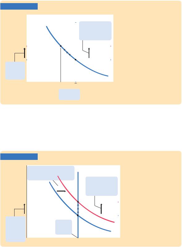
If the money supply is held constant, the increase in velocity causes nominal spending to rise and the aggregate demand curve to shift outward, as in Figure 9-13. In the short run, the increase in demand raises the output of the economy—it causes an economic boom. At the old prices, firms now sell more output. Therefore, they hire more workers, ask their existing workers to work longer hours, and make greater use of their factories and equipment.
Over time, the high level of aggregate demand pulls up wages and prices. As the price level rises, the quantity of output demanded declines, and the economy gradually approaches the natural level of production. But during the transition to the higher price level, the economy’s output is higher than its natural level.
FIGURE 9-13
Price level, P
LRAS
|
|
3. ... but in the |
|
|
|
long run affects |
|
|
|
only the price level. |
|
|
C |
2. ... raises |
|
1. A rise in |
output in |
|
the short |
|
aggregate |
|
run ... |
|
|
demand ... |
|
|
|
|
|
A |
B |
SRAS |
|
|
|
AD2 |
|
|
|
AD1 |
An Increase in Aggregate Demand The economy begins in long-run equilibrium at point A. An increase in aggregate demand, perhaps due to an increase in the velocity of money, moves the economy from point A to point B, where output is above its natural level. As prices rise, output gradually returns
to its natural level, and the economy moves from point B to point C.
280 | P A R T I V Business Cycle Theory: The Economy in the Short Run
What can the Fed do to dampen this boom and keep output closer to the natural level? The Fed might reduce the money supply to offset the increase in velocity. Offsetting the change in velocity would stabilize aggregate demand. Thus, the Fed can reduce or even eliminate the impact of demand shocks on output and employment if it can skillfully control the money supply. Whether the Fed in fact has the necessary skill is a more difficult question, which we take up in Chapter 15.
Shocks to Aggregate Supply
Shocks to aggregate supply can also cause economic fluctuations. A supply shock is a shock to the economy that alters the cost of producing goods and services and, as a result, the prices that firms charge. Because supply shocks have a direct impact on the price level, they are sometimes called price shocks. Here are some examples:
■A drought that destroys crops. The reduction in food supply pushes up food prices.
■A new environmental protection law that requires firms to reduce their emissions of pollutants. Firms pass on the added costs to customers in the form of higher prices.
■An increase in union aggressiveness. This pushes up wages and the prices of the goods produced by union workers.
■The organization of an international oil cartel. By curtailing competition, the major oil producers can raise the world price of oil.
All these events are adverse supply shocks, which means they push costs and prices upward. A favorable supply shock, such as the breakup of an international oil cartel, reduces costs and prices.
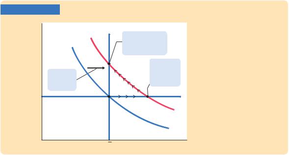
Figure 9-14 shows how an adverse supply shock affects the economy. The short-run aggregate supply curve shifts upward. (The supply shock may also lower the natural level of output and thus shift the long-run aggregate supply curve to the left, but we ignore that effect here.) If aggregate demand is held constant, the economy moves from point A to point B: the price level rises and the amount of output falls below its natural level. An experience like this is called stagflation, because it combines economic stagnation (falling output) with inflation (rising prices).
Faced with an adverse supply shock, a policymaker with the ability to influence aggregate demand, such as the Fed, has a difficult choice between two options. The first option, implicit in Figure 9-14, is to hold aggregate demand constant. In this case, output and employment are lower than the natural level. Eventually, prices will fall to restore full employment at the old price level (point A), but the cost of this adjustment process is a painful recession.
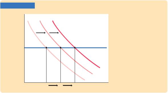
The second option, illustrated in Figure 9-15, is to expand aggregate demand to bring the economy toward the natural level of output more quickly. If the increase in aggregate demand coincides with the shock to aggregate
C H A P T E R 9 Introduction to Economic Fluctuations | 281
Price level, P
2. ... which causes the price level to rise ...
LRAS |
|
|
|
|
1. An adverse supply |
|
|
|
shock shifts the short- |
|
|
|
run aggregate supply |
|
|
|
curve upward, ... |
|
B |
|
SRAS2 |
|
|
|
|
|
|
A |
SRAS1 |
|
|
|
AD |
|
|
|
|
|
 Y Income, output, Y
3. ... and output to fall.
An Adverse Supply Shock An adverse supply shock pushes up costs and thus prices. If aggregate demand is held constant, the economy moves from point A to point B, leading to stagflation—a combination of increasing prices and falling output. Eventually, as prices fall, the economy returns to the natural level of output, point A.
supply, the economy goes immediately from point A to point C. In this case, the Fed is said to accommodate the supply shock. The drawback of this option, of course, is that the price level is permanently higher. There is no way to adjust aggregate demand to maintain full employment and keep the price level stable.
Price level, P
3. ...
resulting in a
permanently higher price level ...
2. ... but the Fed accommodates LRAS the shock by raising aggregate
demand, ...
|
|
|
1. An adverse supply |
|
|
|
shock shifts the short- |
|
|
|
run aggregate supply |
|
|
|
curve upward, ... |
|
|
C |
SRAS2 |
|
|
|
A |
SRAS1 |
|
4. ... but |
AD2 |
no change |
in output. |
AD1 |
|
|
|
|
|
|
|
Income, output, Y |
Y |
Accommodating an Adverse Supply Shock In response to an adverse supply shock, the Fed can increase aggregate demand to prevent a reduction in output. The economy moves from point A to point C. The cost of this policy is a permanently higher level of prices.
282 | P A R T I V Business Cycle Theory: The Economy in the Short Run
CASE STUDY
How OPEC Helped Cause Stagflation in the 1970s and Euphoria in the 1980s
The most disruptive supply shocks in recent history were caused by OPEC, the Organization of Petroleum Exporting Countries. OPEC is a cartel, which is an organization of suppliers that coordinate production levels and prices. In the early 1970s, OPEC’s reduction in the supply of oil nearly doubled the world price. This increase in oil prices caused stagflation in most industrial countries. These statistics show what happened in the United States:
|
Change in |
Inflation |
Unemployment |
Year |
Oil Prices |
Rate (CPI) |
Rate |
1973 |
11.0% |
6.2% |
4.9% |
1974 |
68.0 |
11.0 |
5.6 |
1975 |
16.0 |
9.1 |
8.5 |
1976 |
3.3 |
5.8 |
7.7 |
1977 |
8.1 |
6.5 |
7.1 |
The 68-percent increase in the price of oil in 1974 was an adverse supply shock of major proportions. As one would have expected, this shock led to both higher inflation and higher unemployment.
A few years later, when the world economy had nearly recovered from the first OPEC recession, almost the same thing happened again. OPEC raised oil prices, causing further stagflation. Here are the statistics for the United States:
|
Change in |
Inflation |
Unemployment |
Year |
Oil Prices |
Rate (CPI) |
Rate |
1978 |
9.4% |
7.7% |
6.1% |
1979 |
25.4 |
11.3 |
5.8 |
1980 |
47.8 |
13.5 |
7.0 |
1981 |
44.4 |
10.3 |
7.5 |
1982 |
–8.7 |
6.1 |
9.5 |
The increases in oil prices in 1979, 1980, and 1981 again led to double-digit inflation and higher unemployment.
In the mid-1980s, political turmoil among the Arab countries weakened OPEC’s ability to restrain supplies of oil. Oil prices fell, reversing the stagflation of the 1970s and the early 1980s. Here’s what happened:

|
|
C H A P T E R 9 |
Introduction to Economic Fluctuations | 283 |
|
|
|
|
|
|
Change in |
Inflation |
Unemployment |
Year |
Oil Prices |
Rate (CPI) |
Rate |
1983 |
–7.1% |
3.2% |
9.5% |
|
1984 |
–1.7 |
4.3 |
7.4 |
|
1985 |
–7.5 |
3.6 |
7.1 |
|
1986 |
–44.5 |
1.9 |
6.9 |
|
1987 |
l8.3 |
3.6 |
6.1 |
|
In 1986 oil prices fell by nearly half. This favorable supply shock led to one of the lowest inflation rates experienced in recent U.S. history and to falling unemployment.
More recently, OPEC has not been a major cause of economic fluctuations. Conservation efforts and technological changes have made the U.S. economy less susceptible to oil shocks. The economy today is more service-based and less manufacturing-based, and services typically require less energy to produce than do manufactured goods. Because the amount of oil consumed per unit of real GDP has fallen by more than half over the previous three decades, it takes a much larger oil-price change to have the impact on the economy that we observed in the 1970s and 1980s. Thus, when oil prices rose precipitously in 2007 and the first half of 2008 (before retreating in the second half of 2008), these price changes had a smaller macroeconomic impact than they would have had in the past.5 ■
9-6 Conclusion
This chapter introduced a framework to study economic fluctuations: the model of aggregate supply and aggregate demand. The model is built on the assumption that prices are sticky in the short run and flexible in the long run. It shows how shocks to the economy cause output to deviate temporarily from the level implied by the classical model.
The model also highlights the role of monetary policy. On the one hand, poor monetary policy can be a source of destabilizing shocks to the economy. On the other hand, a well-run monetary policy can respond to shocks and stabilize the economy.
5 Some economists have suggested that changes in oil prices played a major role in economic fluctuations even before the 1970s. See James D. Hamilton, “Oil and the Macroeconomy Since World War II,’’ Journal of Political Economy 91 (April 1983): 228–248.
284 | P A R T I V Business Cycle Theory: The Economy in the Short Run
In the chapters that follow, we refine our understanding of this model and our analysis of stabilization policy. Chapters 10 through 12 go beyond the quantity equation to refine our theory of aggregate demand. Chapter 13 examines aggregate supply in more detail. Chapter 14 brings these elements together in a dynamic model of aggregate demand and aggregate supply. Chapter 15 examines the debate over the virtues and limits of stabilization policy.
Summary
1.Economies experience short-run fluctuations in economic activity, measured most broadly by real GDP. These fluctuations are associated with movement in many macroeconomic variables. In particular, when GDP growth declines, consumption growth falls (typically by a smaller amount), investment growth falls (typically by a larger amount), and unemployment rises. Although economists look at various leading indicators to forecast movements in the economy, these short-run fluctuations are largely unpredictable.
2.The crucial difference between how the economy works in the long run and how it works in the short run is that prices are flexible in the long run but sticky in the short run. The model of aggregate
supply and aggregate demand provides a framework to analyze economic fluctuations and see how the impact of policies and events varies over different time horizons.
3.The aggregate demand curve slopes downward. It tells us that the lower the price level, the greater the aggregate quantity of goods and services demanded.
4.In the long run, the aggregate supply curve is vertical because output is determined by the amounts of capital and labor and by the available technology but not by the level of prices. Therefore, shifts in aggregate demand affect the price level but not output or employment.
5.In the short run, the aggregate supply curve is horizontal, because wages and prices are sticky at predetermined levels. Therefore, shifts in aggregate demand affect output and employment.
6.Shocks to aggregate demand and aggregate supply cause economic fluctuations. Because the Fed can shift the aggregate demand curve, it can attempt to offset these shocks to maintain output and employment at their natural levels.
|
C H A P T E R 9 |
Introduction to Economic Fluctuations | 285 |
K E Y C O N C E P T S |
|
|
|
|
|
Okun’s law |
Aggregate supply |
Supply shocks |
Leading indicators |
Shocks |
Stabilization policy |
Aggregate demand |
Demand shocks |
|
Q U E S T I O N S F O R R E V I E W
1.When real GDP declines during a recession, what typically happens to consumption, investment, and the unemployment rate?
2.Give an example of a price that is sticky in the short run but flexible in the long run.
3.Why does the aggregate demand curve slope downward?
4.Explain the impact of an increase in the money supply in the short run and in the long run.
5.Why is it easier for the Fed to deal with demand shocks than with supply shocks?
P R O B L E M S A N D A P P L I C A T I O N S
1.An economy begins in long-run equilibrium, and then a change in government regulations allows banks to start paying interest on checking accounts. Recall that the money stock is the sum of currency and demand deposits, including checking accounts, so this regulatory change makes holding money more attractive.
a.How does this change affect the demand for money?
b.What happens to the velocity of money?
c.If the Fed keeps the money supply constant, what will happen to output and prices in the short run and in the long run?
d.If the goal of the Fed is to stabilize the price level, should the Fed keep the money supply constant in response to this regulatory change? If not, what should it do? Why?
e.If the goal of the Fed is to stabilize output, how would your answer to part (d) change?
2.Suppose the Fed reduces the money supply by 5 percent.
a.What happens to the aggregate demand curve?
b.What happens to the level of output and the price level in the short run and in the long run?
c.According to Okun’s law, what happens to unemployment in the short run and in the long run?
d.What happens to the real interest rate in the short run and in the long run? (Hint: Use the model of the real interest rate in Chapter 3 to see what happens when output changes.)
3.Let’s examine how the goals of the Fed influence its response to shocks. Suppose Fed A cares only about keeping the price level stable and Fed B cares only about keeping output and employment at their natural levels. Explain how each Fed would respond to the following.
286 | P A R T I V Business Cycle Theory: The Economy in the Short Run
a.An exogenous decrease in the velocity of money.
b.An exogenous increase in the price of oil.
4.The official arbiter of when recessions begin and end is the National Bureau of Economic Research, a nonprofit economics research group. Go to the NBER’s Web site
(www.nber.org) and find the latest turning point in the business cycle. When did it occur? Was this a switch from expansion to contraction or the other way around? List all the recessions (contractions) that have occurred during your lifetime and the dates when they began and ended.

C H A P T E R 10
Aggregate Demand I:
Building the IS–LM Model
I shall argue that the postulates of the classical theory are applicable to a special
case only and not to the general case. . . . Moreover, the characteristics of the
special case assumed by the classical theory happen not to be those of the
economic society in which we actually live, with the result that its teaching is
misleading and disastrous if we attempt to apply it to the facts of experience.
—John Maynard Keynes, The General Theory
Of all the economic fluctuations in world history, the one that stands out as particularly large, painful, and intellectually significant is the Great Depression of the 1930s. During this time, the United States and many other countries experienced massive unemployment and greatly reduced
incomes. In the worst year, 1933, one-fourth of the U.S. labor force was unemployed, and real GDP was 30 percent below its 1929 level.
This devastating episode caused many economists to question the validity of classical economic theory—the theory we examined in Chapters 3 through 6. Classical theory seemed incapable of explaining the Depression. According to that theory, national income depends on factor supplies and the available technology, neither of which changed substantially from 1929 to 1933. After the onset of the Depression, many economists believed that a new model was needed to explain such a large and sudden economic downturn and to suggest government policies that might reduce the economic hardship so many people faced.
In 1936 the British economist John Maynard Keynes revolutionized economics with his book The General Theory of Employment, Interest, and Money.
Keynes proposed a new way to analyze the economy, which he presented as an alternative to classical theory. His vision of how the economy works quickly became a center of controversy. Yet, as economists debated The General Theory, a new understanding of economic fluctuations gradually developed.
Keynes proposed that low aggregate demand is responsible for the low income and high unemployment that characterize economic downturns. He criticized classical theory for assuming that aggregate supply alone—capital, labor, and technology—determines national income. Economists today reconcile
288 | P A R T I V Business Cycle Theory: The Economy in the Short Run
these two views with the model of aggregate demand and aggregate supply introduced in Chapter 9. In the long run, prices are flexible, and aggregate supply determines income. But in the short run, prices are sticky, so changes in aggregate demand influence income. In 2008 and 2009, as the United States and Europe descended into a recession, the Keynesian theory of the business cycle was often in the news. Policymakers around the world debated how best to increase aggregate demand and put their economies on the road to recovery.
In this chapter and the next, we continue our study of economic fluctuations by looking more closely at aggregate demand. Our goal is to identify the variables that shift the aggregate demand curve, causing fluctuations in national income. We also examine more fully the tools policymakers can use to influence aggregate demand. In Chapter 9 we derived the aggregate demand curve from the quantity theory of money, and we showed that monetary policy can shift the aggregate demand curve. In this chapter we see that the government can influence aggregate demand with both monetary and fiscal policy.
The model of aggregate demand developed in this chapter, called the IS–LM model, is the leading interpretation of Keynes’s theory. The goal of the model is to show what determines national income for a given price level. There are two ways to interpret this exercise. We can view the IS –LM model as showing what causes income to change in the short run when the price level is fixed because all prices are sticky. Or we can view the model as showing what causes the aggregate demand curve to shift. These two interpretations of the model are equivalent: as Figure 10-1 shows, in the short run when the price level is fixed, shifts in the aggregate demand curve lead to changes in the equilibrium level of national income.
FIGURE 10-1
Price level, P
AD1 AD2 AD3
Shifts in Aggregate Demand
For a given price level, national income fluctuates because of shifts in the aggregate demand curve. The IS–LM model takes the price level as given and shows what causes income to change. The model therefore shows what causes aggregate demand to shift.
Y1 |
Y2 |
Y3 |
Income, output, Y |