

128 | P A R T I I Classical Theory: The Economy in the Long Run
FIGURE 5-2
Real interest |
S |
|
rate, r |
||
Trade surplus |
||
|
NX
r*
World interest rate
Interest
rate if the
economy I(r) were closed
Investment, Saving, I, S
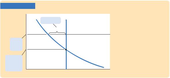
Saving and Investment in a Small Open Economy In a closed economy, the real interest rate adjusts to equilibrate saving and investment. In a small open economy, the interest rate is determined in world financial markets. The difference between saving and investment determines the trade balance. Here there is a trade surplus, because at the world interest rate, saving exceeds investment.
In Chapter 3 we graphed saving and investment as in Figure 5-2. In the closed economy studied in that chapter, the real interest rate adjusts to equilibrate saving and investment—that is, the real interest rate is found where the saving and investment curves cross. In the small open economy, however, the real interest rate equals the world real interest rate. The trade balance is determined by the difference between saving and investment at the world interest rate.
At this point, you might wonder about the mechanism that causes the trade balance to equal the net capital outflow. The determinants of the capital flows are easy to understand. When saving falls short of investment, investors borrow from abroad; when saving exceeds investment, the excess is lent to other countries. But what causes those who import and export to behave so as to ensure that the international flow of goods exactly balances this international flow of capital? For now we leave this question unanswered, but we return to it in Section 5-3 when we discuss the determination of exchange rates.
How Policies Influence the Trade Balance
Suppose that the economy begins in a position of balanced trade. That is, at the world interest rate, investment I equals saving S, and net exports NX equal zero. Let’s use our model to predict the effects of government policies at home and abroad.
Fiscal Policy at Home Consider first what happens to the small open economy if the government expands domestic spending by increasing government purchases. The increase in G reduces national saving, because S = Y − C − G. With an unchanged world real interest rate, investment remains the same. Therefore, saving falls below investment, and some investment must now be financed by borrowing from abroad. Because NX = S − I, the fall in S implies a fall in NX. The economy now runs a trade deficit.
C H A P T E R 5 The Open Economy | 129
FIGURE 5-3
Real interest |
S2 |
S1 |
|
||
rate, r |
2. ... but when a |
||||
|
|
|
|
|
fiscal expansion |
|
|
|
|
|
reduces saving, ... |
|
|
|
|
|
1. This economy |
|
|
|
|
|
begins with |
|
|
|
|
|
balanced trade, ... |
r* |
|
|
|
|
|
|
|
|
NX < 0 |
|
|
|
3. ... a trade |
|
|
|
|
|
deficit results. |
|
|
|
I(r) |
|
|
|
|
|
|
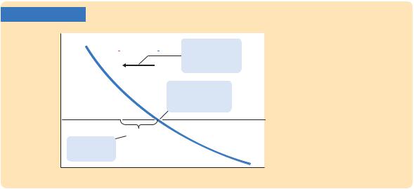
A Fiscal Expansion at Home in a Small Open Economy An increase in government purchases or a reduction in taxes reduces national saving and thus shifts the saving schedule to the left, from S1 to S2. The result is a trade deficit.
Investment, Saving, I, S
The same logic applies to a decrease in taxes. A tax cut lowers T, raises disposable income Y − T, stimulates consumption, and reduces national saving. (Even though some of the tax cut finds its way into private saving, public saving falls by the full amount of the tax cut; in total, saving falls.) Because NX = S − I, the reduction in national saving in turn lowers NX.
Figure 5-3 illustrates these effects. A fiscal policy change that increases private consumption C or public consumption G reduces national saving (Y − C − G ) and, therefore, shifts the vertical line that represents saving from S1 to S2. Because NX is the distance between the saving schedule and the investment schedule at the world interest rate, this shift reduces NX. Hence, starting from balanced trade, a change in fiscal policy that reduces national saving leads to a trade deficit.
Fiscal Policy Abroad Consider now what happens to a small open economy when foreign governments increase their government purchases. If these foreign countries are a small part of the world economy, then their fiscal change has a negligible impact on other countries. But if these foreign countries are a large part of the world economy, their increase in government purchases reduces world saving. The decrease in world saving causes the world interest rate to rise, just as we saw in our closed-economy model (remember, Earth is a closed economy).
The increase in the world interest rate raises the cost of borrowing and, thus, reduces investment in our small open economy. Because there has been no change in domestic saving, saving S now exceeds investment I, and some of our saving begins to flow abroad. Because NX = S − I, the reduction in I must also increase NX. Hence, reduced saving abroad leads to a trade surplus at home.
Figure 5-4 illustrates how a small open economy starting from balanced trade responds to a foreign fiscal expansion. Because the policy change is occurring abroad, the domestic saving and investment schedules remain the same. The only change is an increase in the world interest rate from r*1 to r*2 . The trade balance is the difference between the saving and investment schedules; because
130 | P A R T I I Classical Theory: The Economy in the Long Run
FIGURE 5-4
Real interest
rate, r |
|
S |
||
|
|
|
2. ... reduces |
|
|
|
|
investment |
|
|
|
|
and leads to |
|
|
|
|
a trade surplus. |
|
1. An |
|
NX > 0 |
||
r* |
||||
increase |
||||
2 |
||||
in the |
|
|
|
|
world |
r* |
|||
interest |
1 |
|||
|
|
|||
rate ... |
|
|
||
I(r)
Investment, Saving, I, S
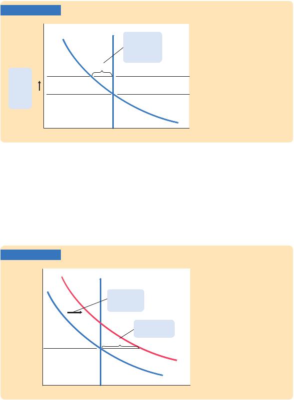
A Fiscal Expansion Abroad in a Small Open Economy A fiscal expansion in a foreign economy large enough to influence world saving and investment raises the world interest rate from r*1 to r*2 . The higher world interest rate reduces investment in this small open economy, causing a trade surplus.
saving exceeds investment at r*2 , there is a trade surplus. Hence, starting from balanced trade, an increase in the world interest rate due to a fiscal expansion abroad leads to a trade surplus.
Shifts in Investment Demand Consider what happens to our small open economy if its investment schedule shifts outward—that is, if the demand for investment goods at every interest rate increases. This shift would occur if, for example, the government changed the tax laws to encourage investment by providing an investment tax credit. Figure 5-5 illustrates the impact of a shift in the
FIGURE 5-5 |
|
|
Real interest |
S |
|
rate, r |
||
|
||
|
1. An increase |
|
|
in investment |
|
|
demand ... |
|
|
2. ... leads to a |
|
|
trade deficit. |
|
r* |
NX < 0 |
|
|
||
|
I(r) |
|
|
2 |
|
|
I(r) |
|
|
1 |
|
|
Investment, Saving, I, S |
A Shift in the Investment Schedule in a Small Open Economy An outward shift in the investment schedule from I(r)1 to I(r)2 increases the amount of investment at the world interest rate r*. As a result, investment now exceeds saving, which means the economy is borrowing from abroad and running a trade deficit.

C H A P T E R 5 The Open Economy | 131
investment schedule. At a given world interest rate, investment is now higher. Because saving is unchanged, some investment must now be financed by borrowing from abroad. Because capital flows into the economy to finance the increased investment, the net capital outflow is negative. Put differently, because
NX = S − I, the increase in I implies a decrease in NX. Hence, starting from balanced trade, an outward shift in the investment schedule causes a trade deficit.
Evaluating Economic Policy
Our model of the open economy shows that the flow of goods and services measured by the trade balance is inextricably connected to the international flow of funds for capital accumulation. The net capital outflow is the difference between domestic saving and domestic investment. Thus, the impact of economic policies on the trade balance can always be found by examining their impact on domestic saving and domestic investment. Policies that increase investment or decrease saving tend to cause a trade deficit, and policies that decrease investment or increase saving tend to cause a trade surplus.
Our analysis of the open economy has been positive, not normative. That is, our analysis of how economic policies influence the international flows of capital and goods has not told us whether these policies are desirable. Evaluating economic policies and their impact on the open economy is a frequent topic of debate among economists and policymakers.
When a country runs a trade deficit, policymakers must confront the question of whether it represents a national problem. Most economists view a trade deficit not as a problem in itself, but perhaps as a symptom of a problem. A trade deficit could be a reflection of low saving. In a closed economy, low saving leads to low investment and a smaller future capital stock. In an open economy, low saving leads to a trade deficit and a growing foreign debt, which eventually must be repaid. In both cases, high current consumption leads to lower future consumption, implying that future generations bear the burden of low national saving.
Yet trade deficits are not always a reflection of an economic malady. When poor rural economies develop into modern industrial economies, they sometimes finance their high levels of investment with foreign borrowing. In these cases, trade deficits are a sign of economic development. For example, South Korea ran large trade deficits throughout the 1970s, and it became one of the success stories of economic growth. The lesson is that one cannot judge economic performance from the trade balance alone. Instead, one must look at the underlying causes of the international flows.
CASE STUDY
The U.S. Trade Deficit
During the 1980s, 1990s, and 2000s, the United States ran large trade deficits. Panel (a) of Figure 5-6 documents this experience by showing net exports as a percentage of GDP. The exact size of the trade deficit fluctuated over time, but
132 | P A R T I I Classical Theory: The Economy in the Long Run
FIGURE 5-6
(a) The U.S. Trade Balance
Percentage of GDP |
2 |
|
|
|
|
|
|
|
|
|
Surplus |
1 |
|
|
|
|
|
|
|
|
|
|
0 |
|
|
|
|
|
|
|
|
|
|
−1 |
|
|
|
|
|
|
|
|
|
|
−2 |
|
|
|
|
|
|
|
|
|
Deficit |
−3 |
|
|
Trade balance |
|
|
|
|
|
|
−4 |
|
|
|
|
|
|
|
|
|
|
|
|
|
|
|
|
|
|
|
|
|
|
−5 |
|
|
|
|
|
|
|
|
|
|
−6 |
|
|
|
|
|
|
|
|
|
|
−7 |
1965 |
1970 |
1975 |
1980 |
1985 |
1990 |
1995 |
2000 |
2005 |
|
1960 |
|||||||||
|
|
|
|
|
|
|
|
|
|
Year |
(b) U.S. Saving and Investment
Percentage of GDP 20 |
|
|
|
|
|
|
|
|
|
19 |
|
|
|
|
|
|
|
|
|
18 |
|
|
|
|
|
Investment |
|
|
|
17 |
|
|
|
|
|
|
|
|
|
16 |
|
|
|
|
|
|
|
|
|
15 |
|
|
|
|
|
|
|
|
|
14 |
|
|
|
|
|
|
|
|
|
13 |
|
|
|
Saving |
|
|
|
|
|
12 |
|
|
|
|
|
|
|
|
|
11 |
|
|
|
|
|
|
|
|
|
10 |
|
|
|
|
|
|
|
|
|
9 |
|
|
|
|
|
|
|
|
|
8 |
1965 |
1970 |
1975 |
1980 |
1985 |
1990 |
1995 |
2000 |
2005 |
1960 |
|||||||||
|
|
|
|
|
|
|
|
|
Year |
The Trade Balance, Saving, and Investment: The U.S. Experience
Panel (a) shows the trade balance as a percentage of GDP. Positive numbers represent a surplus, and negative numbers represent a deficit. Panel (b) shows national saving and investment as a percentage of GDP since 1960. The trade balance equals saving minus investment.
Source: U.S. Department of Commerce.
C H A P T E R 5 The Open Economy | 133
it was large throughout these three decades. In 2007, the trade deficit was $708 billion, or 5.1 percent of GDP. As accounting identities require, this trade deficit had to be financed by borrowing from abroad (or, equivalently, by selling U.S. assets abroad). During this period, the United States went from being the world’s largest creditor to the world’s largest debtor.
What caused the U.S. trade deficit? There is no single explanation. But to understand some of the forces at work, it helps to look at national saving and domestic investment, as shown in panel (b) of the figure. Keep in mind that the trade deficit is the difference between saving and investment.
The start of the trade deficit coincided with a fall in national saving. This development can be explained by the expansionary fiscal policy in the 1980s. With the support of President Reagan, the U.S. Congress passed legislation in 1981 that substantially cut personal income taxes over the next three years. Because these tax cuts were not met with equal cuts in government spending, the federal budget went into deficit. These budget deficits were among the largest ever experienced in a period of peace and prosperity, and they continued long after Reagan left office. According to our model, such a policy should reduce national saving, thereby causing a trade deficit. And, in fact, that is exactly what happened. Because the government budget and trade balance went into deficit at roughly the same time, these shortfalls were called the twin deficits.
Things started to change in the 1990s, when the U.S. federal government got its fiscal house in order. The first President Bush and President Clinton both signed tax increases, while Congress kept a lid on spending. In addition to these policy changes, rapid productivity growth in the late 1990s raised incomes and, thus, further increased tax revenue. These developments moved the U.S. federal budget from deficit to surplus, which in turn caused national saving to rise.
In contrast to what our model predicts, the increase in national saving did not coincide with a shrinking trade deficit, because domestic investment rose at the same time. The likely explanation is that the boom in information technology caused an expansionary shift in the U.S. investment function. Even though fiscal policy was pushing the trade deficit toward surplus, the investment boom was an even stronger force pushing the trade balance toward deficit.
In the early 2000s, fiscal policy once again put downward pressure on national saving. With the second President Bush in the White House, tax cuts were signed into law in 2001 and 2003, while the war on terror led to substantial increases in government spending. The federal government was again running budget deficits. National saving fell to historic lows, and the trade deficit reached historic highs.
A few years later, the trade deficit started to shrink somewhat, as the economy experienced a substantial decline in housing prices (a phenomenon examined in Chapters 11 and 18). Lower housing prices lead to a substantial decline in residential investment. The trade deficit fell from 5.8 percent of GDP at its peak in 2006 to 4.7 percent in 2008.

134 | P A R T I I Classical Theory: The Economy in the Long Run
The history of the U.S. trade deficit shows that this statistic, by itself, does not tell us much about what is happening in the economy. We have to look deeper at saving, investment, and the policies and events that cause them (and thus the trade balance) to change over time.1 ■
CASE STUDY
Why Doesn’t Capital Flow to Poor Countries?
The U.S. trade deficit discussed in the previous Case Study represents a flow of capital into the United States from the rest of the world. What countries were the source of these capital flows? Because the world is a closed economy, the capital must have been coming from those countries that were running trade surpluses. In 2008, this group included many nations that were far poorer than the United States, such as Russia, Malaysia,Venezuela, and China. In these nations, saving exceeded investment in domestic capital. These countries were sending funds abroad to countries like the United States, where investment in domestic capital exceeded saving.
From one perspective, the direction of international capital flows is a paradox. Recall our discussion of production functions in Chapter 3. There, we established that an empirically realistic production function is the Cobb–Douglas form:
F(K,L) = A K aL1−a,
where K is capital, L is labor, A is a variable representing the state of technology, and a is a parameter that determines capital’s share of total income. For this production function, the marginal product of capital is
MPK = a A (K/L)a−1.
The marginal product of capital tells us how much extra output an extra unit of capital would produce. Because a is capital’s share, it must be less than 1, so a − 1 < 0. This means that an increase in K/L decreases MPK. In other words, holding other variables constant, the more capital a nation has, the less valuable an extra unit of capital is. This phenomenon of diminishing marginal product says that capital should be more valuable where capital is scarce.
This prediction, however, seems at odds with the international flow of capital represented by trade imbalances. Capital does not seem to flow to those nations where it should be most valuable. Instead of capital-rich countries like the United States lending to capital-poor countries, we often observe the opposite. Why is that?
One reason is that there are important differences among nations other than their accumulation of capital. Poor nations have not only lower levels of capital accumulation (represented by K/L) but also inferior production capabilities (rep-
1 For more on this topic, see Catherine L. Mann, Is the U.S.Trade Deficit Sustainable? Institute for International Economics, 1999.