350 | P A R T I V Business Cycle Theory: The Economy in the Short Run

the Bretton Woods system—an international monetary system under which most governments agreed to fix exchange rates. The world abandoned this system in the early 1970s, and most exchange rates were allowed to float. Yet fixed exchange rates are not merely of historical interest. More recently, China fixed the value of its currency against the U.S. dollar—a policy that, as we will see, was a source of some tension between the two countries.

In this section we discuss how such a system works, and we examine the impact of economic policies on an economy with a fixed exchange rate. Later in the chapter we examine the pros and cons of fixed exchange rates.

How a Fixed-Exchange-Rate System Works

Under a system of fixed exchange rates, a central bank stands ready to buy or sell the domestic currency for foreign currencies at a predetermined price. For example, suppose the Fed announced that it was going to fix the exchange rate at 100 yen per dollar. It would then stand ready to give $1 in exchange for 100 yen or to give 100 yen in exchange for $1. To carry out this policy, the Fed would need a reserve of dollars (which it can print) and a reserve of yen (which it must have purchased previously).

A fixed exchange rate dedicates a country’s monetary policy to the single goal of keeping the exchange rate at the announced level. In other words, the essence of a fixed-exchange-rate system is the commitment of the central bank to allow the money supply to adjust to whatever level will ensure that the equilibrium exchange rate in the market for foreign-currency exchange equals the announced exchange rate. Moreover, as long as the central bank stands ready to buy or sell foreign currency at the fixed exchange rate, the money supply adjusts automatically to the necessary level.

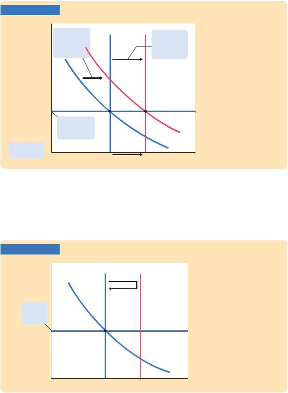
To see how fixing the exchange rate determines the money supply, consider the following example. Suppose the Fed announces that it will fix the exchange rate at 100 yen per dollar, but, in the current equilibrium with the current money supply, the market exchange rate is 150 yen per dollar. This situation is illustrated in panel (a) of Figure 12-7. Notice that there is a profit opportunity: an arbitrageur could buy 300 yen in the foreign-exchange market for $2 and then sell the yen to the Fed for $3, making a $1 profit. When the Fed buys these yen from the arbitrageur, the dollars it pays for them automatically increase the money supply. The rise in the money supply shifts the LM * curve to the right, lowering the equilibrium exchange rate. In this way, the money supply continues to rise until the equilibrium exchange rate falls to the announced level.

Conversely, suppose that when the Fed announces that it will fix the exchange rate at 100 yen per dollar, the equilibrium has a market exchange rate of 50 yen per dollar. Panel (b) of Figure 12-7 shows this situation. In this case, an arbitrageur could make a profit by buying 100 yen from the Fed for $1 and then selling the yen in the marketplace for $2. When the Fed sells these yen, the $1 it receives automatically reduces the money supply. The fall in the money supply shifts the LM* curve to the left, raising the equilibrium exchange rate. The money supply continues to fall until the equilibrium exchange rate rises to the announced level.

C H A P T E R 1 2 The Open Economy Revisited: The Mundell-Fleming Model and the Exchange-Rate Regime | 351

FIGURE 12-7

How a Fixed Exchange Rate Governs the Money Supply In panel (a), the equilibrium exchange rate initially exceeds the fixed level. Arbitrageurs will buy foreign currency in foreign-exchange markets and sell it to the Fed for a profit. This process automatically increases the money supply, shifting the LM* curve to the right and lowering the exchange rate. In panel (b), the equilibrium exchange rate is initially below the fixed level. Arbitrageurs will buy dollars in foreign-exchange markets and use them to buy foreign currency from the Fed. This process automatically reduces the money supply, shifting the LM* curve to the left and raising the exchange rate.

It is important to understand that this exchange-rate system fixes the nominal exchange rate. Whether it also fixes the real exchange rate depends on the time horizon under consideration. If prices are flexible, as they are in the long run, then the real exchange rate can change even while the nominal exchange rate is fixed. Therefore, in the long run described in Chapter 5, a policy to fix the nominal exchange rate would not influence any real variable, including the real exchange rate. A fixed nominal exchange rate would influence only the money supply and the price level. Yet in the short run described by the Mundell–Fleming model, prices are fixed, so a fixed nominal exchange rate implies a fixed real exchange rate as well.

CASE STUDY

The International Gold Standard

During the late nineteenth and early twentieth centuries, most of the world’s major economies operated under the gold standard. Each country maintained a reserve of gold and agreed to exchange one unit of its currency for a specified amount of gold. Through the gold standard, the world’s economies maintained a system of fixed exchange rates.

352 | P A R T I V Business Cycle Theory: The Economy in the Short Run

To see how an international gold standard fixes exchange rates, suppose that the U.S. Treasury stands ready to buy or sell 1 ounce of gold for $100, and the Bank of England stands ready to buy or sell 1 ounce of gold for 100 pounds. Together, these policies fix the rate of exchange between dollars and pounds: $1 must trade for 1 pound. Otherwise, the law of one price would be violated, and it would be profitable to buy gold in one country and sell it in the other.

For example, suppose that the market exchange rate is 2 pounds per dollar. In this case, an arbitrageur could buy 200 pounds for $100, use the pounds to buy 2 ounces of gold from the Bank of England, bring the gold to the United States, and sell it to the Treasury for $200—making a $100 profit. Moreover, by bringing the gold to the United States from England, the arbitrageur would increase the money supply in the United States and decrease the money supply in England.

Thus, during the era of the gold standard, the international transport of gold by arbitrageurs was an automatic mechanism adjusting the money supply and stabilizing exchange rates. This system did not completely fix exchange rates, because shipping gold across the Atlantic was costly. Yet the international gold standard did keep the exchange rate within a range dictated by transportation costs. It thereby prevented large and persistent movements in exchange rates.3 ■

Fiscal Policy

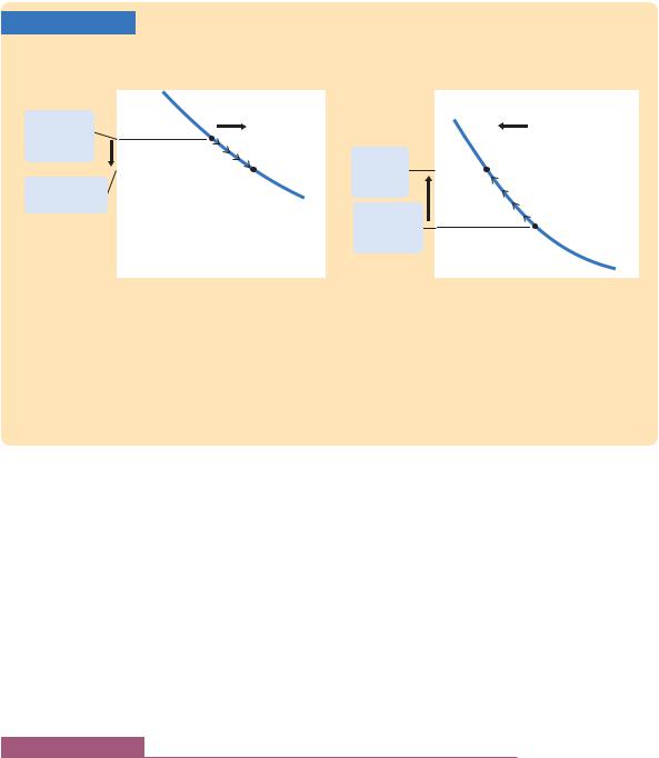
Let’s now examine how economic policies affect a small open economy with a fixed exchange rate. Suppose that the government stimulates domestic spending by increasing government purchases or by cutting taxes. This policy shifts the IS* curve to the right, as in Figure 12-8, putting upward pressure on the market exchange rate. But because the central bank stands ready to trade foreign and domestic currency at the fixed exchange rate, arbitrageurs quickly respond to the rising exchange rate by selling foreign currency to the central bank, leading to an automatic monetary expansion. The rise in the money supply shifts the LM* curve to the right. Thus, under a fixed exchange rate, a fiscal expansion raises aggregate income.

Monetary Policy

Imagine that a central bank operating with a fixed exchange rate tries to increase the money supply—for example, by buying bonds from the public. What would happen? The initial impact of this policy is to shift the LM* curve to the right, lowering the exchange rate, as in Figure 12-9. But, because the central bank is committed to trading foreign and domestic currency at a fixed exchange rate, arbitrageurs quickly respond to the falling exchange rate by selling the domestic

3 For more on how the gold standard worked, see the essays in Barry Eichengreen, ed., The Gold Standard in Theory and History (New York: Methuen, 1985).