Добавил:
Upload Опубликованный материал нарушает ваши авторские права? Сообщите нам.
Вуз: Предмет: Файл:
0554541_86F5E_mankiw_n_gregory_macroeconomics.pdf
Скачиваний:
411
Добавлен:
16.03.2015
Размер:
3.88 Mб
Скачать

C H A P T E R 1 4 A Dynamic Model of Aggregate Demand and Aggregate Supply | 427

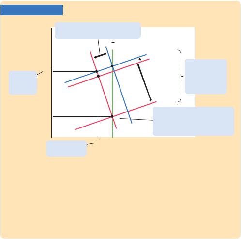
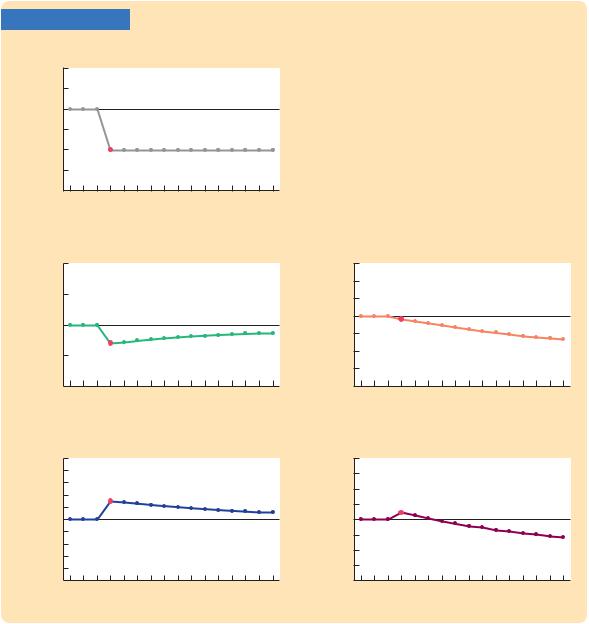
nearby FYI box for their description.) As panel (a) shows, the shock ut spikes upward by 1 percentage point in period t and then returns to zero in subsequent periods. Inflation, shown in panel (d), rises by 0.9 percentage point and gradually returns to its target of 2 percent over a long period of time. Output, shown in panel (b), falls in response to the supply shock but also eventually returns to its natural level.

The figure also shows the paths of nominal and real interest rates. In the period of the supply shock, the nominal interest rate, shown in panel (e), increases by 1.2 percentage points, and the real interest rate, in panel (c), increases by 0.3 percentage points. Both interest rates return to their normal values as the economy returns to its long-run equilibrium.

These figures illustrate the phenomenon of stagflation in the dynamic AD –AS model. A supply shock causes inflation to rise, which in turn increases expected inflation. As the central bank applies its rule for monetary policy and responds by raising interest rates, it gradually squeezes inflation out of the system, but only at the cost of a prolonged downturn in economic activity.

A Shock to Aggregate Demand

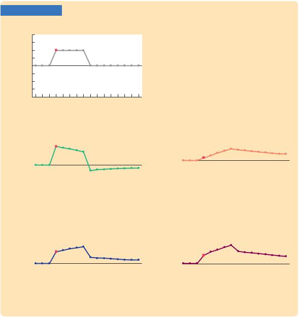
Now let’s consider a shock to aggregate demand. To be realistic, the shock is assumed to persist over several periods. In particular, suppose that et =1 for five periods and then returns to its normal value of zero. This positive shock et might represent, for example, a war that increases government purchases or a stock market bubble that increases wealth and thereby consumption spending.

In general, the demand shock captures any event that influences the demand

for goods and services for given values of the natural level of output Yt and the real interest rate rt.

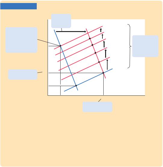
Figure 14-8 shows the result. In period t, when the shock occurs, the dynamic aggregate demand curve shifts to the right from DADt −1 to DADt. Because the demand shock et is not a variable in the dynamic aggregate supply equation, the DAS curve is unchanged from period t − 1 to period t. The economy moves along the dynamic aggregate supply curve from point A to point B. Output and inflation both increase.

Once again, these effects work in part through the reaction of monetary policy to the shock. When the demand shock causes output and inflation to rise, the central bank responds by increasing the nominal and real interest rates. Because a higher real interest rate reduces the quantity of goods and services demanded, it partly offsets the expansionary effects of the demand shock.

In the periods after the shock occurs, expected inflation is higher because expectations depend on past inflation. As a result, the dynamic aggregate supply curve shifts upward repeatedly; as it does so, it continually reduces output and increases inflation. In the figure, the economy goes from point B in the initial period of the shock to points C, D, E, and F in subsequent periods.

In the sixth period (t + 5), the demand shock disappears. At this time, the dynamic aggregate demand curve returns to its initial position. However, the

428 | P A R T I V Business Cycle Theory: The Economy in the Short Run

FIGURE 14-8

Inflation, p

5. When the demand shock disappears, output falls, and

the economy begins

its return to its pt + 5 initial equilibrium.

3. . . . and inflation

pt

to rise.


pt – 1

1. A positive shock to demand . . .

G

Yt + 5


Y

all

DASt + 5


DASt + 4


F


DASt + 3

4. In subsequent


periods, higher


E


DASt + 2


expected inflation


shifts the DAS


D


DASt + 1

curve upward.


C

DASt – 1, t


B


DADt…t + 4


A


DADt – 1, t + 5…


Yt – 1

Yt

Income, output, Y


2. . . . causes output


to increase . . .


A Demand Shock This figure shows the effects of a positive demand shock in period t that lasts for five periods. The shock immediately shifts the dynamic aggregate demand curve to the right from DADt −1 to DADt. The economy moves from point A to point B. Both inflation and output rise. In the next period, the dynamic aggregate supply curve shifts to DASt +1 because of increased expected inflation. The economy moves from point B to point C, and then in subsequent periods to points D, E, and F. When the demand shock disappears after five periods, the dynamic aggregate demand curve shifts back to its initial position, and the economy moves from point F to point G. Output falls below its natural level, and inflation starts to fall. Over time, the dynamic aggregate supply curve starts shifting downward, and the economy gradually returns to its initial equilibrium, point A.

economy does not immediately return to its initial equilibrium, point A. The period of high demand has increased inflation and thereby expected inflation. High expected inflation keeps the dynamic aggregate supply curve higher than it was initially. As a result, when demand falls off, the economy’s equilibrium moves to point G, and output falls to Yt +5, which is below its natural level. The economy then gradually recovers, as the higher-than-target inflation is squeezed out of the system.

Figure 14-9 shows the time path of the key variables in the model in response to the demand shock. Note that the positive demand shock increases real and nominal interest rates. When the demand shock disappears, both interest rates fall. These responses occur because when the central bank sets the nominal interest rate, it takes into account both inflation rates and deviations of output from its natural level.

C H A P T E R 1 4 A Dynamic Model of Aggregate Demand and Aggregate Supply | 429

FIGURE 14-9

(a) Demand Shock

The Dynamic Response to a Demand

et

2.0


1.5


1.0


0.5


0.0


–0.5


–1.0


–1.5


–2.0

t

t + 2 t + 4 t + 6 t + 8 t + 10 t + 12


t – 2


Time

Shock This figure shows the responses of the key variables over time to a positive 1-percent demand shock that lasts for five periods.


(b) Output


(d) Inflation

Yt 101.0


pt 3.5%


100.5


3.0


2.5


100.0


2.0


1.5


99.5


1.0


0.5


99.0


0.0


t – 2 t t + 2 t + 4 t + 6 t + 8 t + 10 t + 12


t – 2 t t + 2 t + 4 t + 6 t + 8 t + 10 t + 12


Time


Time


(c) Real Interest Rate


(e) Nominal Interest Rate

rt 3.0%


it 6.0%


2.8


5.5


2.6


5.0


2.4


4.5


2.2


2.0


4.0


1.8


3.5


1.6


3.0


1.4


2.5


1.2


1.0


2.0


t – 2 t t + 2 t + 4 t + 6 t + 8 t + 10 t + 12


t – 2 t t + 2 t + 4 t + 6 t + 8 t + 10 t + 12


Time


Time

A Shift in Monetary Policy

Suppose that the central bank decides to reduce its target for the inflation rate.

Specifically, imagine that, in period t, p* falls from 2 percent to 1 percent and

t

thereafter remains at that lower level. Let’s consider how the economy will react to this change in monetary policy.

Recall that the inflation target enters the model as an exogenous variable in the dynamic aggregate demand curve. When the inflation target falls, the DAD

430 | P A R T I V Business Cycle Theory: The Economy in the Short Run

curve shifts to the left, as shown in Figure 14-10. (To be precise, it shifts downward by exactly 1 percentage point.) Because target inflation does not enter the dynamic aggregate supply equation, the DAS curve does not shift initially. The economy moves from its initial equilibrium, point A, to a new equilibrium, point

B.Output and inflation both fall.

Monetary policy is, not surprisingly, key to the explanation of this outcome.

When the central bank lowers its target for inflation, current inflation is now above the target, so the central bank follows its policy rule and raises real and nominal interest rates. The higher real interest rate reduces the demand for goods and services. When output falls, the Phillips curve tells us that inflation falls as well.

Lower inflation, in turn, reduces the inflation rate that people expect to prevail in the next period. In period t + 1, lower expected inflation shifts the dynamic aggregate supply curve downward, to DASt +1. (To be precise, the curve shifts downward by exactly the fall in expected inflation.) This shift moves the economy from point B to point C, further reducing inflation and expanding output. Over time, as inflation continues to fall and the DAS curve continues to shift

FIGURE 14-10

Inflation, p

pt – 1 = 2% pt

3. . . . and inflation to fall as well.

pfinal = 1%

1. A reduction in target inflation shifts the DAD curve downward, . . .

Yall

DASt – 1, t


A

DASt + 1

4. In subsequent

B


periods, lower

C


expected inflation


shifts the DAS


curve downward.


DASfinal


5. Eventually, the economy


Z

approaches a final equilibrium, with


DADt – 1

output at its natural level and


inflation at its new, lower target.


DADt, t + 1…


2. . . . causing

Yt Yt – 1 =

Income, output, Y

output to fall . . .

Yfinal


A Reduction in Target Inflation A permanent reduction in target inflation in period t shifts the dynamic aggregate demand curve to the left from DADt −1 to DADt, t +1, . . . . Initially, the economy moves from point A to point B. Both inflation and output fall. In the subsequent period, because expected inflation falls, the dynamic aggregate supply curve shifts downward. The economy moves from point B to point C in period t + 1. Over time, as expected inflation falls and the dynamic aggregate supply curve repeatedly shifts downward, the economy approachesa new equilibrium at point Z. Output returns to its natural level Yall, and

inflation ends at its new, lower target (p*, + = 1 percent).

t t 1, . . .


C H A P T E R 1 4 A Dynamic Model of Aggregate Demand and Aggregate Supply | 431

toward DAS

final

, the economy approaches a new long-run equilibrium at point


Z, where output is back at its natural level (Yfinal = Yall) and inflation is at its new

lower target (p*, + = 1 percent).

t t 1, . . .

Figure 14-11 shows the response of the variables over time to a reduction in target inflation. Note in panel (e) the time path of the nominal interest rate it. Before the change in policy, the nominal interest rate is at its long-run value of 4.0 percent

(which equals the natural real interest rate r of 2 percent plus target inflation p*

t 1

of 2 percent). When target inflation falls to 1 percent, the nominal interest rate rises

FIGURE 14-11

(a) Inflation Target

pt*

3.0


2.5


2.0


1.5


1.0


0.5


0.0

t

t + 2 t + 4 t + 6 t + 8 t + 10 t + 12


t – 2


Time

(b) Output

Yt 101.0

100.5

100.0

99.5

99.0

t – 2

t

t + 2 t + 4 t + 6 t + 8 t + 10 t + 12

Time

(c) Real Interest Rate

rt 3.0% 2.8

2.6

2.4

2.2

2.0

1.8

1.6

1.4

1.2

1.0

t – 2

t

t + 2 t + 4 t + 6 t + 8 t + 10 t + 12

Time

The Dynamic Response to a Reduction in Target Inflation This figure shows the responses of the key variables over time to a permanent reduction in the target rate of inflation.

(d) Inflation

pt

3.5%


3.0


2.5


2.0


1.5


1.0


0.5


0.0

t

t + 2 t + 4 t + 6 t + 8 t + 10 t + 12


t – 2


Time

(e) Nominal Interest Rate

it

6.0%


5.5


5.0


4.5


4.0


3.5


3.0


2.5


2.0

t

t + 2 t + 4 t + 6 t + 8 t + 10 t + 12


t – 2


Time

432 | P A R T I V Business Cycle Theory: The Economy in the Short Run

to 4.2 percent. Over time, however, the nominal interest rate falls as inflation and expected inflation fall toward the new target rate; eventually, it approaches its new long-run value of 3.0 percent. Thus, a shift toward a lower inflation target increases the nominal interest rate in the short run but decreases it in the long run.

We close with a caveat: Throughout this analysis we have maintained the assumption of adaptive expectations. That is, we have assumed that people form their expectations of inflation based on the inflation they have recently experienced. It is possible, however, that if the central bank makes a credible announcement of its new policy of lower target inflation, people will respond by altering their expectations of inflation immediately. That is, they may form expectations rationally, based on the policy announcement, rather than adaptively, based on what they have experienced. (We discussed this possibility in Chapter 13.) If so, the dynamic aggregate supply curve will shift downward immediately upon the change in policy, just when the dynamic aggregate demand curve shifts downward. In this case, the economy will instantly reach its new long-run equilibrium. By contrast, if people do not believe an announced policy of low inflation until they see it, then the assumption of adaptive expectations is appropriate, and the transition path to lower inflation will involve a period of lost output, as shown in Figure 14-11.

14-4 Two Applications: Lessons

for Monetary Policy

So far in this chapter, we have assembled a dynamic model of inflation and output and used it to show how various shocks affect the time paths of output, inflation, and interest rates. We now use the model to shed light on the design of monetary policy.

It is worth pausing at this point to consider what we mean by the phrase “the design of monetary policy.” So far in this analysis, the central bank has had a simple role: it merely had to adjust the money supply to ensure that the nominal interest rate hit the target level prescribed by the monetary-policy rule. The two key parameters of that policy rule are vp (the responsiveness of the target interest rate to inflation) and vY (the responsiveness of the target interest rate to output). We have taken these parameters as given without discussing how they are chosen. Now that we know how the model works, we can consider a deeper question: what should the parameters of the monetary policy rule be?

The Tradeoff Between Output Variability

and Inflation Variability

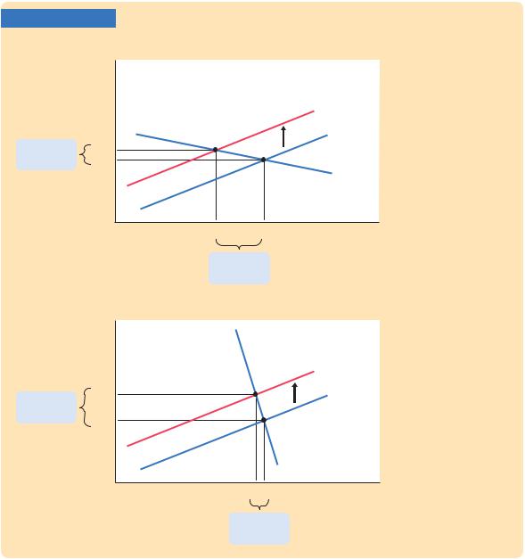
Consider the impact of a supply shock on output and inflation. According to the dynamic AD –AS model, the impact of this shock depends crucially on the slope of the dynamic aggregate demand curve. In particular, the slope of the DAD curve determines whether a supply shock has a large or small impact on output and inflation.

C H A P T E R 1 4 A Dynamic Model of Aggregate Demand and Aggregate Supply | 433

This phenomenon is illustrated in Figure 14-12. In the two panels of this figure, the economy experiences the same supply shock. In panel (a), the dynamic aggregate demand curve is nearly flat, so the shock has a small effect on inflation but a large effect on output. In panel (b), the dynamic aggregate demand curve is steep, so the shock has a large effect on inflation but a small effect on output.

Why is this important for monetary policy? Because the central bank can influence the slope of the dynamic aggregate demand curve. Recall the equation for the DAD curve:

= − − av av p p* av e

Yt Yt [ p/(1 + Y)]( t t ) + [1/(1 + Y)] t.

FIGURE 14-12

(a) DAD Curve Is Flat

Inflation, p


DASt


B


DASt – 1

Small change

A


pt


in inflation

pt – 1


DADt – 1, t


Yt

Yt – 1

Income, output, Y

Large change in output

(b) DAD Curve Is Steep

Inflation, p


DASt


B′

DASt – 1

Large change

pt


A′


in inflation

pt – 1


DADt – 1, t


Yt

Yt – 1

Income, output, Y

Two Possible Responses to a Supply Shock When the dynamic aggregate demand curve is relatively flat, as in panel (a), a supply shock has a small effect on inflation but a large effect on output. When the dynamic aggregate demand curve is relatively steep, as in panel (b), the same supply shock has a large effect on inflation but a small effect on output. The slope of the dynamic aggregate demand curve is based in part on the parameters of monetary policy (vp and vY), which describe how much interest rates respond to changes in inflation and output. When choosing these parameters, the central bank faces a tradeoff between the variability of inflation and the variability of output.

Small change in output

434 | P A R T I V Business Cycle Theory: The Economy in the Short Run

Two key parameters here are vp and vY, which govern how much the central bank’s interest rate target responds to changes in inflation and output. When the central bank chooses these policy parameters, it determines the slope of the DAD curve and thus the economy’s short-run response to supply shocks.

On the one hand, suppose that, when setting the interest rate, the central bank responds strongly to inflation (vp is large) and weakly to output (vY is small). In this case, the coefficient on inflation in the above equation is large. That is, a small change in inflation has a large effect on output. As a result, the dynamic aggregate demand curve is relatively flat, and supply shocks have large effects on output but small effects on inflation. The story goes like this: When the economy experiences a supply shock that pushes up inflation, the central bank’s policy rule has it respond vigorously with higher interest rates. Sharply higher interest rates significantly reduce the quantity of goods and services demanded, thereby leading to a large recession that dampens the inflationary impact of the shock (which was the purpose of the monetary policy response).

On the other hand, suppose that, when setting the interest rate, the central bank responds weakly to inflation (vp is small) but strongly to output (vY is large). In this case, the coefficient on inflation in the above equation is small, which means that even a large change in inflation has only a small effect on output. As a result, the dynamic aggregate demand curve is relatively steep, and supply shocks have small effects on output but large effects on inflation. The story is just the opposite as before: Now, when the economy experiences a supply shock that pushes up inflation, the central bank’s policy rule has it respond with only slightly higher interest rates. This small policy response avoids a large recession but accommodates the inflationary shock.

In its choice of monetary policy, the central bank determines which of these two scenarios will play out. That is, when setting the policy parameters vp and vY , the central bank chooses whether to make the economy look more like panel (a) or more like panel (b) of Figure 14-12. When making this choice, the central bank faces a tradeoff between output variability and inflation variability. The central bank can be a hard-line inflation fighter, as in panel (a), in which case inflation is stable but output is volatile. Alternatively, it can be more accommodative, as in panel (b), in which case inflation is volatile but output is more stable. It can also choose some position in between these two extremes.

One job of a central bank is to promote economic stability. There are, however, various dimensions to this charge. When there are tradeoffs to be made, the central bank has to determine what kind of stability to pursue. The dynamic AD –AS model shows that one fundamental tradeoff is between the variability in inflation and the variability in output.

Note that this tradeoff is very different from a simple tradeoff between inflation and output. In the long run of this model, inflation goes to its target, and output goes to its natural level. Consistent with classical macroeconomic theory, policymakers do not face a long-run tradeoff between inflation and output. Instead, they face a choice about which of these two measures of

C H A P T E R 1 4 A Dynamic Model of Aggregate Demand and Aggregate Supply | 435

macroeconomic performance they want to stabilize. When deciding on the parameters of the monetary-policy rule, they determine whether supply shocks lead to inflation variability, output variability, or some combination of the two.

CASE STUDY

The Fed Versus the European Central Bank

According to the dynamic AD –AS model, a key policy choice facing any central bank concerns the parameters of its policy rule. The monetary parameters vp and vY determine how much the interest rate responds to macroeconomic conditions. As we have just seen, these responses in turn determine the volatility of inflation and output.

The U.S. Federal Reserve and the European Central Bank (ECB) appear to have different approaches to this decision. The legislation that created the Fed states explicitly that its goal is “to promote effectively the goals of maximum employment, stable prices, and moderate long-term interest rates.” Because the Fed is supposed to stabilize both employment and prices, it is said to have a dual mandate. (The third goal—moderate long-term interest rates—should follow naturally from stable prices.) By contrast, the ECB says on its Web site that “the primary objective of the ECB’s monetary policy is to maintain price stability. The ECB aims at inflation rates of below, but close to, 2% over the medium term.” All other macroeconomic goals, including stability of output and employment, appear to be secondary.

We can interpret these differences in light of our model. Compared to the Fed, the ECB seems to give more weight to inflation stability and less weight to output stability. This difference in objectives should be reflected in the parameters of the monetary-policy rules. To achieve its dual mandate, the Fed would respond more to output and less to inflation than the ECB would.

A case in point occurred in 2008 when the world economy was experiencing rising oil prices, a financial crisis, and a slowdown in economic activity. The Fed responded to these events by lowering interest rates from about 5 percent to a range of 0 to 0.25 percent over the course of a year. The ECB, facing a similar situation, also cut interest rates—but by much less. The ECB was less concerned about recession and more concerned about keeping inflation in check.

The dynamic AD–AS model predicts that, other things equal, the policy of the ECB should, over time, lead to more variable output and more stable inflation. Testing this prediction, however, is difficult for two reasons. First, because the ECB was established only in 1998, there is not yet enough data to establish the longterm effects of its policy. Second, and perhaps more important, other things are not always equal. Europe and the United States differ in many ways beyond the policies of their central banks, and these other differences may affect output and inflation in ways unrelated to differences in monetary-policy priorities.