- •About the author
- •Brief Contents
- •Contents
- •Preface
- •This Book’s Approach
- •What’s New in the Seventh Edition?
- •The Arrangement of Topics
- •Part One, Introduction
- •Part Two, Classical Theory: The Economy in the Long Run
- •Part Three, Growth Theory: The Economy in the Very Long Run
- •Part Four, Business Cycle Theory: The Economy in the Short Run
- •Part Five, Macroeconomic Policy Debates
- •Part Six, More on the Microeconomics Behind Macroeconomics
- •Epilogue
- •Alternative Routes Through the Text
- •Learning Tools
- •Case Studies
- •FYI Boxes
- •Graphs
- •Mathematical Notes
- •Chapter Summaries
- •Key Concepts
- •Questions for Review
- •Problems and Applications
- •Chapter Appendices
- •Glossary
- •Translations
- •Acknowledgments
- •Supplements and Media
- •For Instructors
- •Instructor’s Resources
- •Solutions Manual
- •Test Bank
- •PowerPoint Slides
- •For Students
- •Student Guide and Workbook
- •Online Offerings
- •EconPortal, Available Spring 2010
- •eBook
- •WebCT
- •BlackBoard
- •Additional Offerings
- •i-clicker
- •The Wall Street Journal Edition
- •Financial Times Edition
- •Dismal Scientist
- •1-1: What Macroeconomists Study
- •1-2: How Economists Think
- •Theory as Model Building
- •The Use of Multiple Models
- •Prices: Flexible Versus Sticky
- •Microeconomic Thinking and Macroeconomic Models
- •1-3: How This Book Proceeds
- •Income, Expenditure, and the Circular Flow
- •Rules for Computing GDP
- •Real GDP Versus Nominal GDP
- •The GDP Deflator
- •Chain-Weighted Measures of Real GDP
- •The Components of Expenditure
- •Other Measures of Income
- •Seasonal Adjustment
- •The Price of a Basket of Goods
- •The CPI Versus the GDP Deflator
- •The Household Survey
- •The Establishment Survey
- •The Factors of Production
- •The Production Function
- •The Supply of Goods and Services
- •3-2: How Is National Income Distributed to the Factors of Production?
- •Factor Prices
- •The Decisions Facing the Competitive Firm
- •The Firm’s Demand for Factors
- •The Division of National Income
- •The Cobb–Douglas Production Function
- •Consumption
- •Investment
- •Government Purchases
- •Changes in Saving: The Effects of Fiscal Policy
- •Changes in Investment Demand
- •3-5: Conclusion
- •4-1: What Is Money?
- •The Functions of Money
- •The Types of Money
- •The Development of Fiat Money
- •How the Quantity of Money Is Controlled
- •How the Quantity of Money Is Measured
- •4-2: The Quantity Theory of Money
- •Transactions and the Quantity Equation
- •From Transactions to Income
- •The Assumption of Constant Velocity
- •Money, Prices, and Inflation
- •4-4: Inflation and Interest Rates
- •Two Interest Rates: Real and Nominal
- •The Fisher Effect
- •Two Real Interest Rates: Ex Ante and Ex Post
- •The Cost of Holding Money
- •Future Money and Current Prices
- •4-6: The Social Costs of Inflation
- •The Layman’s View and the Classical Response
- •The Costs of Expected Inflation
- •The Costs of Unexpected Inflation
- •One Benefit of Inflation
- •4-7: Hyperinflation
- •The Costs of Hyperinflation
- •The Causes of Hyperinflation
- •4-8: Conclusion: The Classical Dichotomy
- •The Role of Net Exports
- •International Capital Flows and the Trade Balance
- •International Flows of Goods and Capital: An Example
- •Capital Mobility and the World Interest Rate
- •Why Assume a Small Open Economy?
- •The Model
- •How Policies Influence the Trade Balance
- •Evaluating Economic Policy
- •Nominal and Real Exchange Rates
- •The Real Exchange Rate and the Trade Balance
- •The Determinants of the Real Exchange Rate
- •How Policies Influence the Real Exchange Rate
- •The Effects of Trade Policies
- •The Special Case of Purchasing-Power Parity
- •Net Capital Outflow
- •The Model
- •Policies in the Large Open Economy
- •Conclusion
- •Causes of Frictional Unemployment
- •Public Policy and Frictional Unemployment
- •Minimum-Wage Laws
- •Unions and Collective Bargaining
- •Efficiency Wages
- •The Duration of Unemployment
- •Trends in Unemployment
- •Transitions Into and Out of the Labor Force
- •6-5: Labor-Market Experience: Europe
- •The Rise in European Unemployment
- •Unemployment Variation Within Europe
- •The Rise of European Leisure
- •6-6: Conclusion
- •7-1: The Accumulation of Capital
- •The Supply and Demand for Goods
- •Growth in the Capital Stock and the Steady State
- •Approaching the Steady State: A Numerical Example
- •How Saving Affects Growth
- •7-2: The Golden Rule Level of Capital
- •Comparing Steady States
- •The Transition to the Golden Rule Steady State
- •7-3: Population Growth
- •The Steady State With Population Growth
- •The Effects of Population Growth
- •Alternative Perspectives on Population Growth
- •7-4: Conclusion
- •The Efficiency of Labor
- •The Steady State With Technological Progress
- •The Effects of Technological Progress
- •Balanced Growth
- •Convergence
- •Factor Accumulation Versus Production Efficiency
- •8-3: Policies to Promote Growth
- •Evaluating the Rate of Saving
- •Changing the Rate of Saving
- •Allocating the Economy’s Investment
- •Establishing the Right Institutions
- •Encouraging Technological Progress
- •The Basic Model
- •A Two-Sector Model
- •The Microeconomics of Research and Development
- •The Process of Creative Destruction
- •8-5: Conclusion
- •Increases in the Factors of Production
- •Technological Progress
- •The Sources of Growth in the United States
- •The Solow Residual in the Short Run
- •9-1: The Facts About the Business Cycle
- •GDP and Its Components
- •Unemployment and Okun’s Law
- •Leading Economic Indicators
- •9-2: Time Horizons in Macroeconomics
- •How the Short Run and Long Run Differ
- •9-3: Aggregate Demand
- •The Quantity Equation as Aggregate Demand
- •Why the Aggregate Demand Curve Slopes Downward
- •Shifts in the Aggregate Demand Curve
- •9-4: Aggregate Supply
- •The Long Run: The Vertical Aggregate Supply Curve
- •From the Short Run to the Long Run
- •9-5: Stabilization Policy
- •Shocks to Aggregate Demand
- •Shocks to Aggregate Supply
- •10-1: The Goods Market and the IS Curve
- •The Keynesian Cross
- •The Interest Rate, Investment, and the IS Curve
- •How Fiscal Policy Shifts the IS Curve
- •10-2: The Money Market and the LM Curve
- •The Theory of Liquidity Preference
- •Income, Money Demand, and the LM Curve
- •How Monetary Policy Shifts the LM Curve
- •Shocks in the IS–LM Model
- •From the IS–LM Model to the Aggregate Demand Curve
- •The IS–LM Model in the Short Run and Long Run
- •11-3: The Great Depression
- •The Spending Hypothesis: Shocks to the IS Curve
- •The Money Hypothesis: A Shock to the LM Curve
- •Could the Depression Happen Again?
- •11-4: Conclusion
- •12-1: The Mundell–Fleming Model
- •The Goods Market and the IS* Curve
- •The Money Market and the LM* Curve
- •Putting the Pieces Together
- •Fiscal Policy
- •Monetary Policy
- •Trade Policy
- •How a Fixed-Exchange-Rate System Works
- •Fiscal Policy
- •Monetary Policy
- •Trade Policy
- •Policy in the Mundell–Fleming Model: A Summary
- •12-4: Interest Rate Differentials
- •Country Risk and Exchange-Rate Expectations
- •Differentials in the Mundell–Fleming Model
- •Pros and Cons of Different Exchange-Rate Systems
- •The Impossible Trinity
- •12-6: From the Short Run to the Long Run: The Mundell–Fleming Model With a Changing Price Level
- •12-7: A Concluding Reminder
- •Fiscal Policy
- •Monetary Policy
- •A Rule of Thumb
- •The Sticky-Price Model
- •Implications
- •Adaptive Expectations and Inflation Inertia
- •Two Causes of Rising and Falling Inflation
- •Disinflation and the Sacrifice Ratio
- •13-3: Conclusion
- •14-1: Elements of the Model
- •Output: The Demand for Goods and Services
- •The Real Interest Rate: The Fisher Equation
- •Inflation: The Phillips Curve
- •Expected Inflation: Adaptive Expectations
- •The Nominal Interest Rate: The Monetary-Policy Rule
- •14-2: Solving the Model
- •The Long-Run Equilibrium
- •The Dynamic Aggregate Supply Curve
- •The Dynamic Aggregate Demand Curve
- •The Short-Run Equilibrium
- •14-3: Using the Model
- •Long-Run Growth
- •A Shock to Aggregate Supply
- •A Shock to Aggregate Demand
- •A Shift in Monetary Policy
- •The Taylor Principle
- •14-5: Conclusion: Toward DSGE Models
- •15-1: Should Policy Be Active or Passive?
- •Lags in the Implementation and Effects of Policies
- •The Difficult Job of Economic Forecasting
- •Ignorance, Expectations, and the Lucas Critique
- •The Historical Record
- •Distrust of Policymakers and the Political Process
- •The Time Inconsistency of Discretionary Policy
- •Rules for Monetary Policy
- •16-1: The Size of the Government Debt
- •16-2: Problems in Measurement
- •Measurement Problem 1: Inflation
- •Measurement Problem 2: Capital Assets
- •Measurement Problem 3: Uncounted Liabilities
- •Measurement Problem 4: The Business Cycle
- •Summing Up
- •The Basic Logic of Ricardian Equivalence
- •Consumers and Future Taxes
- •Making a Choice
- •16-5: Other Perspectives on Government Debt
- •Balanced Budgets Versus Optimal Fiscal Policy
- •Fiscal Effects on Monetary Policy
- •Debt and the Political Process
- •International Dimensions
- •16-6: Conclusion
- •Keynes’s Conjectures
- •The Early Empirical Successes
- •The Intertemporal Budget Constraint
- •Consumer Preferences
- •Optimization
- •How Changes in Income Affect Consumption
- •Constraints on Borrowing
- •The Hypothesis
- •Implications
- •The Hypothesis
- •Implications
- •The Hypothesis
- •Implications
- •17-7: Conclusion
- •18-1: Business Fixed Investment
- •The Rental Price of Capital
- •The Cost of Capital
- •The Determinants of Investment
- •Taxes and Investment
- •The Stock Market and Tobin’s q
- •Financing Constraints
- •Banking Crises and Credit Crunches
- •18-2: Residential Investment
- •The Stock Equilibrium and the Flow Supply
- •Changes in Housing Demand
- •18-3: Inventory Investment
- •Reasons for Holding Inventories
- •18-4: Conclusion
- •19-1: Money Supply
- •100-Percent-Reserve Banking
- •Fractional-Reserve Banking
- •A Model of the Money Supply
- •The Three Instruments of Monetary Policy
- •Bank Capital, Leverage, and Capital Requirements
- •19-2: Money Demand
- •Portfolio Theories of Money Demand
- •Transactions Theories of Money Demand
- •The Baumol–Tobin Model of Cash Management
- •19-3 Conclusion
- •Lesson 2: In the short run, aggregate demand influences the amount of goods and services that a country produces.
- •Question 1: How should policymakers try to promote growth in the economy’s natural level of output?
- •Question 2: Should policymakers try to stabilize the economy?
- •Question 3: How costly is inflation, and how costly is reducing inflation?
- •Question 4: How big a problem are government budget deficits?
- •Conclusion
- •Glossary
- •Index
496 | P A R T V I More on the Microeconomics Behind Macroeconomics
17-1 John Maynard Keynes and the
Consumption Function
We begin our study of consumption with John Maynard Keynes’s General Theory, which was published in 1936. Keynes made the consumption function central to his theory of economic fluctuations, and it has played a key role in macroeconomic analysis ever since. Let’s consider what Keynes thought about the consumption function and then see what puzzles arose when his ideas were confronted with the data.
Keynes’s Conjectures
Today, economists who study consumption rely on sophisticated techniques of data analysis. With the help of computers, they analyze aggregate data on the behavior of the overall economy from the national income accounts and detailed data on the behavior of individual households from surveys. Because Keynes wrote in the 1930s, however, he had neither the advantage of these data nor the computers necessary to analyze such large data sets. Instead of relying on statistical analysis, Keynes made conjectures about the consumption function based on introspection and casual observation.
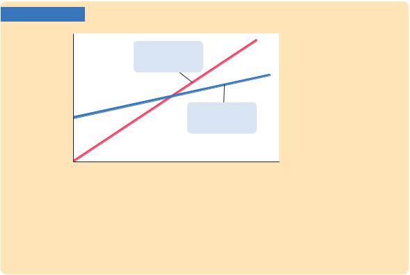
First and most important, Keynes conjectured that the marginal propensity to consume—the amount consumed out of an additional dollar of income—is between zero and one. He wrote that the “fundamental psychological law, upon which we are entitled to depend with great confidence, . . . is that men are disposed, as a rule and on the average, to increase their consumption as their income increases, but not by as much as the increase in their income.’’That is, when a person earns an extra dollar, he typically spends some of it and saves some of it. As we saw in Chapter 10 when we developed the Keynesian cross, the marginal propensity to consume was crucial to Keynes’s policy recommendations for how to reduce widespread unemployment.The power of fiscal policy to influence the economy—as expressed by the fiscal-policy multipliers—arises from the feedback between income and consumption.
Second, Keynes posited that the ratio of consumption to income, called the average propensity to consume, falls as income rises. He believed that saving was a luxury, so he expected the rich to save a higher proportion of their income than the poor.Although not essential for Keynes’s own analysis, the postulate that the average propensity to consume falls as income rises became a central part of early Keynesian economics.
Third, Keynes thought that income is the primary determinant of consumption and that the interest rate does not have an important role.This conjecture stood in stark contrast to the beliefs of the classical economists who preceded him.The classical economists held that a higher interest rate encourages saving and discourages consumption. Keynes admitted that the interest rate could influence consumption as a matter of theory.Yet he wrote that “the main conclusion suggested by experience, I think, is that the short-period influence of the rate of interest on individual spending out of a given income is secondary and relatively unimportant.’’
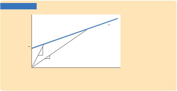
C H A P T E R 1 7 Consumption | 497
On the basis of these three conjectures, the Keynesian consumption function
is often written as |
|
|
|
|
|
− |
+ cY, |
− |
> 0, 0 < c |
< 1, |
|
C = C |
C |
||||
|
|
|
− |
is a constant, and c is the |
|
where C is consumption, Y is disposable income, C |
|
marginal propensity to consume. This consumption function, shown in Figure
−
17-1, is graphed as a straight line. C determines the intercept on the vertical axis, and c determines the slope.
Notice that this consumption function exhibits the three properties that Keynes posited. It satisfies Keynes’s first property because the marginal propensity to consume c is between zero and one, so that higher income leads to higher consumption and also to higher saving. This consumption function satisfies Keynes’s second property because the average propensity to consume APC is
= = − +
APC C/Y C/Y c.
−
As Y rises, C /Y falls, and so the average propensity to consume C/Y falls. And finally, this consumption function satisfies Keynes’s third property because the interest rate is not included in this equation as a determinant of consumption.
The Early Empirical Successes
Soon after Keynes proposed the consumption function, economists began collecting and examining data to test his conjectures. The earliest studies indicated that the Keynesian consumption function was a good approximation of how consumers behave.
In some of these studies, researchers surveyed households and collected data on consumption and income. They found that households with higher income
FIGURE 17-1
Consumption, C
MPC
1
C
APC
1 APC
1
C = C + cY
Income, Y
The Keynesian Consumption Function
This figure graphs a consumption function with the three properties that Keynes conjectured. First, the marginal propensity to consume c is between zero and one. Second, the average propensity to consume falls as income rises. Third, consumption is determined by current income.
Note: The marginal propensity to consume, MPC, is the slope of the consumption function. The average propensity to consume, APC = C/Y, equals the slope of a line drawn from the origin to a point on the consumption function.
498 | P A R T V I More on the Microeconomics Behind Macroeconomics
consumed more, which confirms that the marginal propensity to consume is greater than zero. They also found that households with higher income saved more, which confirms that the marginal propensity to consume is less than one. In addition, these researchers found that higher-income households saved a larger fraction of their income, which confirms that the average propensity to consume falls as income rises. Thus, these data verified Keynes’s conjectures about the marginal and average propensities to consume.
In other studies, researchers examined aggregate data on consumption and income for the period between the two world wars. These data also supported the Keynesian consumption function. In years when income was unusually low, such as during the depths of the Great Depression, both consumption and saving were low, indicating that the marginal propensity to consume is between zero and one. In addition, during those years of low income, the ratio of consumption to income was high, confirming Keynes’s second conjecture. Finally, because the correlation between income and consumption was so strong, no other variable appeared to be important for explaining consumption. Thus, the data also confirmed Keynes’s third conjecture that income is the primary determinant of how much people choose to consume.
Secular Stagnation, Simon Kuznets,
and the Consumption Puzzle
Although the Keynesian consumption function met with early successes, two anomalies soon arose. Both concern Keynes’s conjecture that the average propensity to consume falls as income rises.
The first anomaly became apparent after some economists made a dire—and, it turned out, erroneous—prediction during World War II. On the basis of the Keynesian consumption function, these economists reasoned that as incomes in the economy grew over time, households would consume a smaller and smaller fraction of their incomes.They feared that there might not be enough profitable investment projects to absorb all this saving. If so, the low consumption would lead to an inadequate demand for goods and services, resulting in a depression once the wartime demand from the government ceased. In other words, on the basis of the Keynesian consumption function, these economists predicted that the economy would experience what they called secular stagnation—a long depression of indefinite duration—unless the government used fiscal policy to expand aggregate demand.
Fortunately for the economy, but unfortunately for the Keynesian consumption function, the end of World War II did not throw the country into another depression. Although incomes were much higher after the war than before, these higher incomes did not lead to large increases in the rate of saving. Keynes’s conjecture that the average propensity to consume would fall as income rose appeared not to hold.
The second anomaly arose when economist Simon Kuznets constructed new aggregate data on consumption and income dating back to 1869. Kuznets assembled these data in the 1940s and would later receive the Nobel Prize for this
C H A P T E R 1 7 Consumption | 499
work. He discovered that the ratio of consumption to income was remarkably stable from decade to decade, despite large increases in income over the period he studied. Again, Keynes’s conjecture that the average propensity to consume would fall as income rose appeared not to hold.
The failure of the secular-stagnation hypothesis and the findings of Kuznets both indicated that the average propensity to consume is fairly constant over long periods of time. This fact presented a puzzle that motivated much of the subsequent research on consumption. Economists wanted to know why some studies confirmed Keynes’s conjectures and others refuted them. That is, why did Keynes’s conjectures hold up well in the studies of household data and in the studies of short time-series but fail when long time-series were examined?
Figure 17-2 illustrates the puzzle.The evidence suggested that there were two consumption functions. For the household data and for the short time-series, the Keynesian consumption function appeared to work well. Yet for the long time-series, the consumption function appeared to exhibit a constant average propensity to consume. In Figure 17-2, these two relationships between consumption and income are called the short-run and long-run consumption functions. Economists needed to explain how these two consumption functions could be consistent with each other.
In the 1950s, Franco Modigliani and Milton Friedman each proposed explanations of these seemingly contradictory findings. Both economists later won Nobel Prizes, in part because of their work on consumption. But before we see
FIGURE 17-2
Consumption, C
Long-run consumption function (constant APC)
Short-run consumption function (falling APC)
Income, Y
The Consumption Puzzle
Studies of household data and short time-series found a relationship between consumption and income similar to the one Keynes conjectured. In the figure, this relationship is called the short-run consumption function. But studies of long time-series found that the average propensity to consume did not vary systematically with income. This relationship is called the long-run consumption function. Notice that the short-run consumption function has a falling average propensity to consume, whereas the long-run consumption function has a constant average propensity to consume.