318 | P A R T I V Business Cycle Theory: The Economy in the Short Run

TA B L E 11-1

The Fiscal-Policy Multipliers in the DRI Model

Note: This table gives the fiscal-policy multipliers for a sustained change in government purchases or in personal income taxes. These multipliers are for the fourth quarter after the policy change is made.

Source: Otto Eckstein, The DRI Model of the U.S. Economy (New York: McGraw-Hill, 1983), 169.

That is, a $100 billion increase in government purchases raises GDP by $60 billion, and a $100 billion increase in taxes lowers GDP by $26 billion.

Table 11-1 shows that the fiscal-policy multipliers are very different under the two assumptions about monetary policy. The impact of any change in fiscal policy depends crucially on how the Fed responds to that change. ■

Shocks in the IS–LM Model

Because the IS–LM model shows how national income is determined in the short run, we can use the model to examine how various economic disturbances affect income. So far we have seen how changes in fiscal policy shift the IS curve and how changes in monetary policy shift the LM curve. Similarly, we can group other disturbances into two categories: shocks to the IS curve and shocks to the LM curve.

Shocks to the IS curve are exogenous changes in the demand for goods and services. Some economists, including Keynes, have emphasized that such changes in demand can arise from investors’ animal spirits—exogenous and perhaps self-fulfilling waves of optimism and pessimism. For example, suppose that firms become pessimistic about the future of the economy and that this pessimism causes them to build fewer new factories. This reduction in the demand for investment goods causes a contractionary shift in the investment function: at every interest rate, firms want to invest less. The fall in investment reduces planned expenditure and shifts the IS curve to the left, reducing income and employment. This fall in equilibrium income in part validates the firms’ initial pessimism.

Shocks to the IS curve may also arise from changes in the demand for consumer goods. Suppose, for instance, that the election of a popular president increases consumer confidence in the economy. This induces consumers to save less for the future and consume more today. We can interpret this change as an upward shift in the consumption function. This shift in the consumption function increases planned expenditure and shifts the IS curve to the right, and this raises income.

Shocks to the LM curve arise from exogenous changes in the demand for money. For example, suppose that new restrictions on credit-card availability increase the amount of money people choose to hold. According to the theory

C H A P T E R 1 1 Aggregate Demand II: Applying the IS-LM Model | 319

of liquidity preference, when money demand rises, the interest rate necessary to equilibrate the money market is higher (for any given level of income and money supply). Hence, an increase in money demand shifts the LM curve upward, which tends to raise the interest rate and depress income.

In summary, several kinds of events can cause economic fluctuations by shifting the IS curve or the LM curve. Remember, however, that such fluctuations are not inevitable. Policymakers can try to use the tools of monetary and fiscal policy to offset exogenous shocks. If policymakers are sufficiently quick and skillful (admittedly, a big if ), shocks to the IS or LM curves need not lead to fluctuations in income or employment.

CASE STUDY

The U.S. Recession of 2001

In 2001, the U.S. economy experienced a pronounced slowdown in economic activity. The unemployment rate rose from 3.9 percent in September 2000 to 4.9 percent in August 2001, and then to 6.3 percent in June 2003. In many ways, the slowdown looked like a typical recession driven by a fall in aggregate demand.

Three notable shocks explain this event. The first was a decline in the stock market. During the 1990s, the stock market experienced a boom of historic proportions, as investors became optimistic about the prospects of the new information technology. Some economists viewed the optimism as excessive at the time, and in hindsight this proved to be the case. When the optimism faded, average stock prices fell by about 25 percent from August 2000 to August 2001. The fall in the market reduced household wealth and thus consumer spending. In addition, the declining perceptions of the profitability of the new technologies led to a fall in investment spending. In the language of the IS–LM model, the IS curve shifted to the left.

The second shock was the terrorist attacks on New York City and Washington, D.C., on September 11, 2001. In the week after the attacks, the stock market fell another 12 percent, which at the time was the biggest weekly loss since the Great Depression of the 1930s. Moreover, the attacks increased uncertainty about what the future would hold. Uncertainty can reduce spending because households and firms postpone some of their plans until the uncertainty is resolved. Thus, the terrorist attacks shifted the IS curve farther to the left.

320 | P A R T I V Business Cycle Theory: The Economy in the Short Run

The third shock was a series of accounting scandals at some of the nation’s most prominent corporations, including Enron and WorldCom. The result of these scandals was the bankruptcy of some companies that had fraudulently represented themselves as more profitable than they truly were, criminal convictions for the executives who had been responsible for the fraud, and new laws aimed at regulating corporate accounting standards more thoroughly. These events further depressed stock prices and discouraged business investment—a third leftward shift in the IS curve.

Fiscal and monetary policymakers responded quickly to these events. Congress passed a major tax cut in 2001, including an immediate tax rebate, and a second major tax cut in 2003. One goal of these tax cuts was to stimulate consumer spending. (See the Case Study on cutting taxes in Chapter 10.) In addition, after the terrorist attacks, Congress increased government spending by appropriating funds to assist in New York’s recovery and to bail out the ailing airline industry. These fiscal measures shifted the IS curve to the right.

At the same time, the Federal Reserve pursued expansionary monetary policy, shifting the LM curve to the right. Money growth accelerated, and interest rates fell. The interest rate on three-month Treasury bills fell from 6.4 percent in November 2000 to 3.3 percent in August 2001, just before the terrorist attacks. After the attacks and corporate scandals hit the economy, the Fed increased its monetary stimulus, and the Treasury bill rate fell to 0.9 percent in July 2003— the lowest level in many decades.

Expansionary monetary and fiscal policy had the intended effects. Economic growth picked up in the second half of 2003 and was strong throughout 2004. By July 2005, the unemployment rate was back down to 5.0 percent, and it stayed at or below that level for the next several years. Unemployment would begin rising again in 2008, however, when the economy experienced another recession. The causes of the 2008 recession are examined in another case study later in this chapter. ■

What Is the Fed’s Policy Instrument—The Money

Supply or the Interest Rate?

Our analysis of monetary policy has been based on the assumption that the Fed influences the economy by controlling the money supply. By contrast, when the media report on changes in Fed policy, they often just say that the Fed has raised or lowered interest rates. Which is right? Even though these two views may seem different, both are correct, and it is important to understand why.

In recent years, the Fed has used the federal funds rate—the interest rate that banks charge one another for overnight loans—as its short-term policy instrument. When the Federal Open Market Committee meets every six weeks to set monetary policy, it votes on a target for this interest rate that will apply until the next meeting. After the meeting is over, the Fed’s bond traders (who are located in New York) are told to conduct the open-market operations necessary to hit that target. These openmarket operations change the money supply and shift the LM curve so that the equilibrium interest rate (determined by the intersection of the IS and LM curves) equals the target interest rate that the Federal Open Market Committee has chosen.

As a result of this operating procedure, Fed policy is often discussed in terms of changing interest rates. Keep in mind, however, that behind these changes in

C H A P T E R 1 1 Aggregate Demand II: Applying the IS-LM Model | 321

interest rates are the necessary changes in the money supply. A newspaper might report, for instance, that “the Fed has lowered interest rates.” To be more precise, we can translate this statement as meaning “the Federal Open Market Committee has instructed the Fed bond traders to buy bonds in open-market operations so as to increase the money supply, shift the LM curve, and reduce the equilibrium interest rate to hit a new lower target.”

Why has the Fed chosen to use an interest rate, rather than the money supply, as its short-term policy instrument? One possible answer is that shocks to the LM curve are more prevalent than shocks to the IS curve. When the Fed targets interest rates, it automatically offsets LM shocks by adjusting the money supply, although this policy exacerbates IS shocks. If LM shocks are the more prevalent type, then a policy of targeting the interest rate leads to greater economic stability than a policy of targeting the money supply. (Problem 7 at the end of this chapter asks you to analyze this issue more fully.)

In Chapter 14 we extend our theory of short-run fluctuations to include explicitly a monetary policy that targets the interest rate and that changes its target in response to economic conditions. The IS –LM model presented here is a useful foundation for that more complicated and realistic analysis. One lesson from the IS –LM model is that when a central bank sets the money supply, it determines the equilibrium interest rate. Thus, in some ways, setting the money supply and setting the interest rate are two sides of the same coin.

11-2 IS–LM as a Theory of

Aggregate Demand

We have been using the IS –LM model to explain national income in the short run when the price level is fixed. To see how the IS –LM model fits into the model of aggregate supply and aggregate demand introduced in Chapter 9, we now examine what happens in the IS –LM model if the price level is allowed to change. By examining the effects of changing the price level, we can finally deliver what was promised when we began our study of the IS –LM model: a theory to explain the position and slope of the aggregate demand curve.

From the IS–LM Model to the Aggregate Demand Curve

Recall from Chapter 9 that the aggregate demand curve describes a relationship between the price level and the level of national income. In Chapter 9 this relationship was derived from the quantity theory of money. That analysis showed that for a given money supply, a higher price level implies a lower level of income. Increases in the money supply shift the aggregate demand curve to the right, and decreases in the money supply shift the aggregate demand curve to the left.

To understand the determinants of aggregate demand more fully, we now use the IS –LM model, rather than the quantity theory, to derive the aggregate demand curve. First, we use the IS –LM model to show why national income falls as the price level rises—that is, why the aggregate demand curve is downward sloping. Second, we examine what causes the aggregate demand curve to shift.

322 | P A R T I V Business Cycle Theory: The Economy in the Short Run

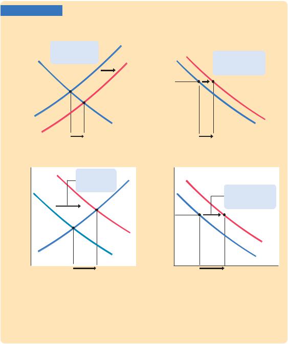
To explain why the aggregate demand curve slopes downward, we examine what happens in the IS–LM model when the price level changes. This is done in Figure 11-5. For any given money supply M, a higher price level P reduces the supply of real money balances M/P. A lower supply of real money balances shifts the LM curve upward, which raises the equilibrium interest rate and lowers the equilibrium level of income, as shown in panel (a). Here the price level rises from P1 to P2, and income falls from Y1 to Y2. The aggregate demand curve in panel (b) plots this negative relationship between national income and the price level. In other words, the aggregate demand curve shows the set of equilibrium points that arise in the IS–LM model as we vary the price level and see what happens to income.

What causes the aggregate demand curve to shift? Because the aggregate demand curve summarizes the results from the IS–LM model, events that shift the IS curve or the LM curve (for a given price level) cause the aggregate demand curve to shift. For instance, an increase in the money supply raises income in the IS–LM model for any given price level; it thus shifts the aggregate demand curve to the right, as shown in panel (a) of Figure 11-6. Similarly, an increase in government purchases or a decrease in taxes raises income in the IS–LM model for a given price level; it also shifts the aggregate demand curve to the right, as shown in panel (b) of Figure 11-6. Conversely, a decrease in the money supply, a decrease in government purchases, or an increase in taxes lowers income in the IS–LM model and shifts the aggregate demand curve to the left. Anything that changes income in the IS–LM model other than a change in the price level causes a shift

FIGURE 11-5

P1

2. ... lowering income Y.

Deriving the Aggregate Demand Curve with the IS–LM Model Panel (a) shows the IS–LM model: an increase in the price level from P1 to P2 lowers real money balances and thus shifts the LM curve upward. The shift in the LM curve lowers income from Y1 to Y2. Panel (b) shows the aggregate demand curve summarizing this relationship between the price level and income: the higher the price level, the lower the level of income.