298 | P A R T I V Business Cycle Theory: The Economy in the Short Run

areas are also declining because they have been producing goods and services that are not in great demand, and will not be in demand in the future. Therefore, the overall value added by improving their roads and other infrastructure is likely to be a lot less than if the new infrastructure were located in growing areas that might have relatively little unemployment, but do have great demand for more roads, schools, and other types of long-term infrastructure.

While Congress debated these and other concerns, President Obama responded to critics of the bill as follows:“So then you get the argument, well, this is not a stimulus bill, this is a spending bill. What do you think a stimulus is? That’s the whole point. No, seriously. That’s the point.” The logic here is quintessentially Keynesian: as the economy sinks into recession, the government is acting as the demander of last resort.

In the end, Congress went ahead with President Obama’s proposed stimulus plans with relatively minor modifications. The president signed the $787 billion bill on February 17, 2009. ■

The Interest Rate, Investment, and the IS Curve

The Keynesian cross is only a stepping-stone on our path to the IS –LM model, which explains the economy’s aggregate demand curve. The Keynesian cross is useful because it shows how the spending plans of households, firms, and the government determine the economy’s income. Yet it makes the simplifying assumption that the level of planned investment I is fixed. As we discussed in Chapter 3, an important macroeconomic relationship is that planned investment depends on the interest rate r.

To add this relationship between the interest rate and investment to our model, we write the level of planned investment as

I = I(r).

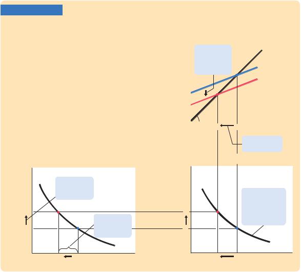
This investment function is graphed in panel (a) of Figure 10-7. Because the interest rate is the cost of borrowing to finance investment projects, an increase in the interest rate reduces planned investment. As a result, the investment function slopes downward.

To determine how income changes when the interest rate changes, we can combine the investment function with the Keynesian-cross diagram. Because investment is inversely related to the interest rate, an increase in the interest rate from r1 to r2 reduces the quantity of investment from I(r1) to I(r2). The reduction in planned investment, in turn, shifts the planned-expenditure function downward, as in panel (b) of Figure 10-7. The shift in the planned-expenditure function causes the level of income to fall from Y1 to Y2. Hence, an increase in the interest rate lowers income.

The IS curve, shown in panel (c) of Figure 10-7, summarizes this relationship between the interest rate and the level of income. In essence, the IS curve combines the interaction between r and I expressed by the investment function and the interaction between I and Y demonstrated by the Keynesian cross. Each point on the IS curve represents equilibrium in the goods market, and the curve illus-

C H A P T E R 1 0 Aggregate Demand I: Building the IS–LM Model | 299

FIGURE 10-7

trates how the equilibrium level of income depends on the interest rate. Because an increase in the interest rate causes planned investment to fall, which in turn causes equilibrium income to fall, the IS curve slopes downward.

How Fiscal Policy Shifts the IS Curve

The IS curve shows us, for any given interest rate, the level of income that brings the goods market into equilibrium. As we learned from the Keynesian cross, the equilibrium level of income also depends on government spending G and taxes T. The IS curve is drawn for a given fiscal policy; that is, when we construct the IS curve, we hold G and T fixed. When fiscal policy changes, the IS curve shifts.

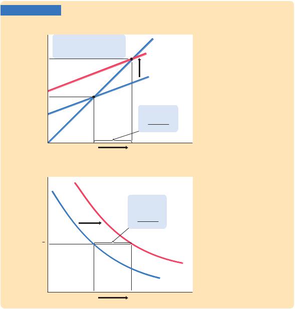
Figure 10-8 uses the Keynesian cross to show how an increase in government purchases G shifts the IS curve. This figure is drawn for a given interest rate r−