530 | P A R T V I More on the Microeconomics Behind Macroeconomics

This equation states that the cost of capital depends on the price of capital, the real interest rate, and the depreciation rate.

Finally, we want to express the cost of capital relative to other goods in the economy. The real cost of capital—the cost of buying and renting out a unit of capital measured in units of the economy’s output—is

Real Cost of Capital = (PK/P)(r + d).

This equation states that the real cost of capital depends on the relative price of a capital good PK/P, the real interest rate r, and the depreciation rate d.

The Determinants of Investment

Now consider a rental firm’s decision about whether to increase or decrease its capital stock. For each unit of capital, the firm earns real revenue R/P and bears the real cost (PK/P)(r + d). The real profit per unit of capital is

Because the real rental price in equilibrium equals the marginal product of capital, we can write the profit rate as

Profit Rate = MPK − (PK/P)(r + d).

The rental firm makes a profit if the marginal product of capital is greater than the cost of capital. It incurs a loss if the marginal product is less than the cost of capital.

We can now see the economic incentives that lie behind the rental firm’s investment decision. The firm’s decision regarding its capital stock—that is, whether to add to it or to let it depreciate—depends on whether owning and renting out capital is profitable. The change in the capital stock, called net investment, depends on the difference between the marginal product of capital and the cost of capital. If the marginal product of capital exceeds the cost of capital, firms find it profitable to add to their capital stock. If the marginal product of capital falls short of the cost of capital, they let their capital stock shrink.

We can also now see that the separation of economic activity between production and rental firms, although useful for clarifying our thinking, is not necessary for our conclusion regarding how firms choose how much to invest. For a firm that both uses and owns capital, the benefit of an extra unit of capital is the marginal product of capital, and the cost is the cost of capital. Like a firm that owns and rents out capital, this firm adds to its capital stock if the marginal product exceeds the cost of capital. Thus, we can write

DK = In [MPK − (PK/P)(r + d)],

where In( ) is the function showing how much net investment responds to the incentive to invest.

C H A P T E R 1 8 Investment | 531

We can now derive the investment function. Total spending on business fixed investment is the sum of net investment and the replacement of depreciated capital. The investment function is

I = In [MPK − (PK/P)(r + d)] + dK.

Business fixed investment depends on the marginal product of capital, the cost of capital, and the amount of depreciation.

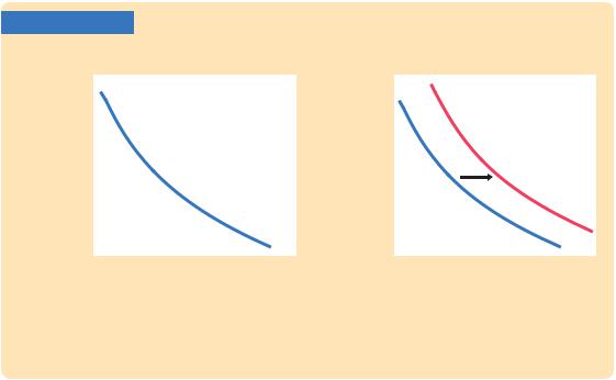
This model shows why investment depends on the interest rate. A decrease in the real interest rate lowers the cost of capital. It therefore raises the amount of profit from owning capital and increases the incentive to accumulate more capital. Similarly, an increase in the real interest rate raises the cost of capital and leads firms to reduce their investment. For this reason, the investment schedule relating investment to the interest rate slopes downward, as in panel (a) of Figure 18-3.

The model also shows what causes the investment schedule to shift. Any event that raises the marginal product of capital increases the profitability of investment and causes the investment schedule to shift outward, as in panel (b) of Figure 18-3. For example, a technological innovation that increases the production function parameter A raises the marginal product of capital and, for any given interest rate, increases the amount of capital goods that rental firms wish to buy.

Finally, consider what happens as this adjustment of the capital stock continues over time. If the marginal product begins above the cost of capital, the capital stock will rise and the marginal product will fall. If the marginal product of capital begins below the cost of capital, the capital stock will fall and the marginal

FIGURE 18-3

The Investment Function Panel (a) shows that business fixed investment increases when the interest rate falls. This is because a lower interest rate reduces the cost of capital and therefore makes owning capital more profitable. Panel (b) shows an outward shift in the investment function, which might be due to an increase in the marginal product of capital.

532 | P A R T V I More on the Microeconomics Behind Macroeconomics

product will rise. Eventually, as the capital stock adjusts, the marginal product of capital approaches the cost of capital. When the capital stock reaches a steady-state level, we can write

MPK = (PK/P)(r + d).

Thus, in the long run, the marginal product of capital equals the real cost of capital. The speed of adjustment toward the steady state depends on how quickly firms adjust their capital stock, which in turn depends on how costly it is to build, deliver, and install new capital.1

Taxes and Investment

Tax laws influence firms’ incentives to accumulate capital in many ways. Sometimes policymakers change the tax code to shift the investment function and influence aggregate demand. Here we consider two of the most important provisions of corporate taxation: the corporate income tax and the investment tax credit.

The corporate income tax is a tax on corporate profits. Throughout much of its history, the corporate tax rate in the United States was 46 percent. The rate was lowered to 34 percent in 1986 and then raised to 35 percent in 1993, and it remained at that level as of 2009, when this book was going to press.

The effect of a corporate income tax on investment depends on how the law defines “profit’’ for the purpose of taxation. Suppose, first, that the law defined profit as we did previously—the rental price of capital minus the cost of capital. In this case, even though firms would be sharing a fraction of their profits with the government, it would still be rational for them to invest if the rental price of capital exceeded the cost of capital and to disinvest if the rental price fell short of the cost of capital. A tax on profit, measured in this way, would not alter investment incentives.

Yet, because of the tax law’s definition of profit, the corporate income tax does affect investment decisions. There are many differences between the law’s definition of profit and ours. For example, one difference is the treatment of depreciation. Our definition of profit deducts the current value of depreciation as a cost. That is, it bases depreciation on how much it would cost today to replace worn-out capital. By contrast, under the corporate tax laws, firms deduct depreciation using historical cost. That is, the depreciation deduction is based on the price of the capital when it was originally purchased. In periods of inflation, replacement cost is greater than historical cost, so the corporate tax tends to understate the cost of depreciation and overstate profit. As a result, the tax law sees a profit and levies a tax even when economic profit is zero, which makes owning capital less attractive. For this and other reasons, many economists believe that the corporate income tax discourages investment.

Policymakers often change the rules governing the corporate income tax in an attempt to encourage investment or at least mitigate the disincentive the tax

1 Economists often measure capital goods in units such that the price of 1 unit of capital equals the price of 1 unit of other goods and services (PK = P ). This was the approach taken implicitly in Chapters 7 and 8, for example. In this case, the steady-state condition says that the marginal product of capital net of depreciation, MPK − d, equals the real interest rate r.

C H A P T E R 1 8 Investment | 533

provides. One example is the investment tax credit, a tax provision that reduces a firm’s taxes by a certain amount for each dollar spent on capital goods. Because a firm recoups part of its expenditure on new capital in lower taxes, the credit reduces the effective purchase price of a unit of capital PK. Thus, the investment tax credit reduces the cost of capital and raises investment.

In 1985 the investment tax credit was 10 percent. Yet the Tax Reform Act of 1986, which reduced the corporate income tax rate, also eliminated the investment tax credit. When Bill Clinton ran for president in 1992, he campaigned on a platform of reinstituting the investment tax credit, but he did not succeed in getting this proposal through Congress. Many economists agreed with Clinton that the investment tax credit is an effective way to stimulate investment, and the idea of reinstating the investment tax credit still arises from time to time.

The tax rules regarding depreciation are another example of how policymakers can influence the incentives for investment. When George W. Bush became president, the economy was sliding into recession, attributable in large measure to a significant decline in business investment. The tax cuts Bush signed into law during his first term included provisions for temporary “bonus depreciation.” This meant that for purposes of calculating their corporate tax liability, firms could deduct the cost of depreciation earlier in the life of an investment project. This bonus, however, was available only for investments made before the end of 2004. The goal of the policy was to encourage investment at a time when the economy particularly needed a boost to aggregate demand. According to a recent study by economists Christopher House and Matthew Shapiro, the goal was achieved to some degree. They write, “While their aggregate effects were probably modest, the 2002 and 2003 bonus depreciation policies had noticeable effects on the economy. For the U.S. economy as a whole, these policies may have increased GDP by $10 to $20 billion and may have been responsible for the creation of 100,000 to 200,000 jobs.”2

The Stock Market and Tobin’s q

Many economists see a link between fluctuations in investment and fluctuations in the stock market. The term stock refers to shares in the ownership of corporations, and the stock market is the market in which these shares are traded. Stock prices tend to be high when firms have many opportunities for profitable investment, because these profit opportunities mean higher future income for the shareholders. Thus, stock prices reflect the incentives to invest.

The Nobel Prize–winning economist James Tobin proposed that firms base their investment decisions on the following ratio, which is now called Tobin’s q:

Market Value of Installed Capital

q = . Replacement Cost of Installed Capital

2 A classic study of how taxes influence investment is Robert E. Hall and Dale W. Jorgenson,“Tax Policy and Investment Behavior,’’ American Economic Review 57 ( June 1967): 391–414. For a study of the recent corporate tax changes, see Christopher L. House and Matthew D. Shapiro, “Temporary Investment Tax Incentives: Theory with Evidence from Bonus Depreciation,’’ NBER Working Paper No. 12514, 2006.

534 | P A R T V I More on the Microeconomics Behind Macroeconomics

The numerator of Tobin’s q is the value of the economy’s capital as determined by the stock market. The denominator is the price of that capital if it were purchased today.

Tobin reasoned that net investment should depend on whether q is greater or less than 1. If q is greater than 1, then the stock market values installed capital at more than its replacement cost. In this case, managers can raise the market value of their firms’ stock by buying more capital. Conversely, if q is less than 1, the stock market values capital at less than its replacement cost. In this case, managers will not replace capital as it wears out.

At first the q theory of investment may appear very different from the neoclassical model developed previously, but the two theories are closely related. To see the relationship, note that Tobin’s q depends on current and future expected profits from installed capital. If the marginal product of capital exceeds the cost of capital, then firms are earning profits on their installed capital. These profits make the firms more desirable to own, which raises the market value of these firms’ stock, implying a high value of q. Similarly, if the marginal product of capital falls short of the cost of capital, then firms are incurring losses on their installed capital, implying a low market value and a low value of q.

The advantage of Tobin’s q as a measure of the incentive to invest is that it reflects the expected future profitability of capital as well as the current profitability. For example, suppose that Congress legislates a reduction in the corporate income tax beginning next year. This expected fall in the corporate tax means greater profits for the owners of capital. These higher expected profits raise the value of stock today, raise Tobin’s q, and therefore encourage investment today. Thus, Tobin’s q theory of investment emphasizes that investment decisions depend not only on current economic policies but also on policies expected to prevail in the future.3

CASE STUDY

The Stock Market as an Economic Indicator

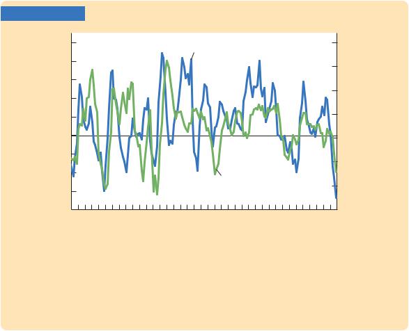
“The stock market has predicted nine out of the last five recessions.” So goes Paul Samuelson’s famous quip about the stock market’s reliability as an economic indicator. The stock market is in fact quite volatile, and it can give false signals about the future of the economy. Yet one should not ignore the link between the stock market and the economy. Figure 18-4 shows that changes in the stock market often reflect changes in real GDP. Whenever the stock market experiences a substantial decline, there is reason to fear that a recession may be around the corner.

Why do stock prices and economic activity tend to fluctuate together? One reason is given by Tobin’s q theory, together with the model of aggregate demand

3 To read more about the relationship between the neoclassical model of investment and q theory, see Fumio Hayashi, “Tobin’s Marginal q and Average q: A Neoclassical Approach,’’ Econometrica 50 ( January 1982): 213–224; and Lawrence H. Summers, “Taxation and Corporate Investment: A q-Theory Approach,’’ Brookings Papers on Economic Activity 1 (1981): 67–140.

The Stock Market and the Economy This figure shows the association between the stock market and real economic activity. Using quarterly data from 1970 to 2008, it presents the percentage change from one year earlier in the Dow Jones Industrial Average (an index of stock prices of major industrial companies) and in real GDP. The figure shows that the stock market and GDP tend to move together but that the association is far from precise.

Source: U.S. Department of Commerce and Global Financial Data.

and aggregate supply. Suppose, for instance, that you observe a fall in stock prices. Because the replacement cost of capital is fairly stable, a fall in the stock market is usually associated with a fall in Tobin’s q. A fall in q reflects investors’ pessimism about the current or future profitability of capital. This means that the investment function has shifted inward: investment is lower at any given interest rate. As a result, the aggregate demand for goods and services contracts, leading to lower output and employment.

There are two additional reasons why stock prices are associated with economic activity. First, because stock is part of household wealth, a fall in stock prices makes people poorer and thus depresses consumer spending, which also reduces aggregate demand. Second, a fall in stock prices might reflect bad news about technological progress and long-run economic growth. If so, this means that the natural level of output—and thus aggregate supply—will be growing more slowly in the future than was previously expected.

These links between the stock market and the economy are not lost on policymakers, such as those at the Federal Reserve. Indeed, because the stock market often anticipates changes in real GDP, and because data on the stock market are available more quickly than data on GDP, the stock market is a closely

536 | P A R T V I More on the Microeconomics Behind Macroeconomics

watched economic indicator. A case in point is the deep economic downturn in 2008 and 2009: the substantial declines in production and employment were preceded by a steep decline in stock prices. ■

Alternative Views of the Stock Market: The Efficient

Markets Hypothesis Versus Keynes’s Beauty Contest

One continuing source of debate among economists is whether stock market fluctuations are rational.

Some economists subscribe to the efficient markets hypothesis, according to which the market price of a company’s stock is the fully rational valuation of the company’s value, given current information about the company’s business prospects. This hypothesis rests on two foundations:

1.Each company listed on a major stock exchange is followed closely by many professional portfolio managers, such as the individuals who run mutual funds. Every day, these managers monitor news stories to try to determine the company’s value. Their job is to buy a stock when its price falls below its value and to sell it when its price rises above its value.

2.The price of each stock is set by the equilibrium of supply and demand. At the market price, the number of shares being offered for sale exactly equals the number of shares that people want to buy. That is, at the market price, the number of people who think the stock is overvalued exactly balances the number of people who think it’s undervalued. As judged by the typical person in the market, the stock must be fairly valued.

According to this theory, the stock market is informationally efficient: it reflects all available information about the value of the asset. Stock prices change when information changes. When good news about the company’s prospects becomes public, the value and the stock price both rise. When the company’s prospects deteriorate, the value and price both fall. But at any moment in time, the market price is the rational best guess of the company’s value based on available information.

One implication of the efficient markets hypothesis is that stock prices should follow a random walk. This means that the changes in stock prices should be impossible to predict from available information. If, based on publicly available information, a person could predict that a stock price would rise by 10 percent tomorrow, then the stock market must be failing to incorporate that information today. According to this theory, the only thing that can move stock prices is news that changes the market’s perception of the company’s value. But such news must be unpredictable—otherwise, it wouldn’t really be news. For the same reason, changes in stock prices should be unpredictable as well.

What is the evidence for the efficient markets hypothesis? Its proponents point out that it is hard to beat the market by buying allegedly undervalued stocks and selling allegedly overvalued stocks. Statistical tests show that stock prices are random walks, or at least approximately so. Moreover, index funds, which buy stocks from all companies in a stock market index, outperform most actively managed mutual funds run by professional money managers.