C H A P T E R 1 2 The Open Economy Revisited: The Mundell-Fleming Model and the Exchange-Rate Regime | 345

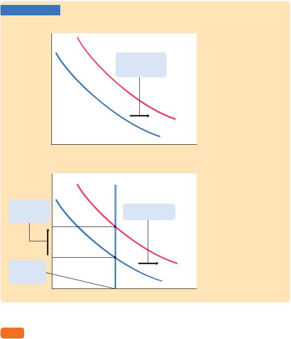
FIGURE 12-3

12-2 The Small Open Economy

Under Floating Exchange Rates

Before analyzing the impact of policies in an open economy, we must specify the international monetary system in which the country has chosen to operate. That is, we must consider how people engaged in international trade and finance can convert the currency of one country into the currency of another.

We start with the system relevant for most major economies today: floating exchange rates. Under a system of floating exchange rates, the exchange rate is set by market forces and is allowed to fluctuate in response to changing economic conditions. In this case, the exchange rate e adjusts to achieve simultaneous equilibrium in the goods market and the money market. When something happens to change that equilibrium, the exchange rate is allowed to move to a new equilibrium value.

Let’s now consider three policies that can change the equilibrium: fiscal policy, monetary policy, and trade policy. Our goal is to use the Mundell–Fleming model to show the impact of policy changes and to understand the economic forces at work as the economy moves from one equilibrium to another.

Fiscal Policy

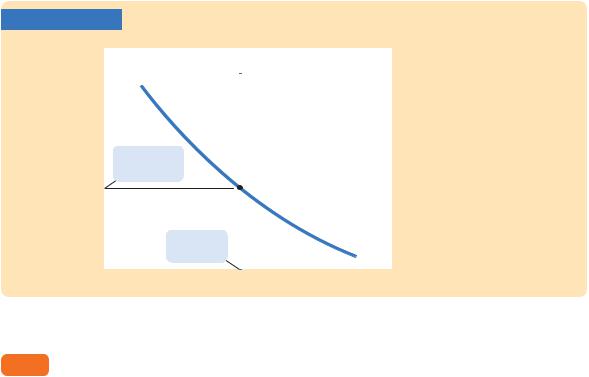
Suppose that the government stimulates domestic spending by increasing government purchases or by cutting taxes. Because such expansionary fiscal policy increases planned expenditure, it shifts the IS* curve to the right, as in Figure 12-4. As a result, the exchange rate appreciates, while the level of income remains the same.

348 | P A R T I V Business Cycle Theory: The Economy in the Short Run

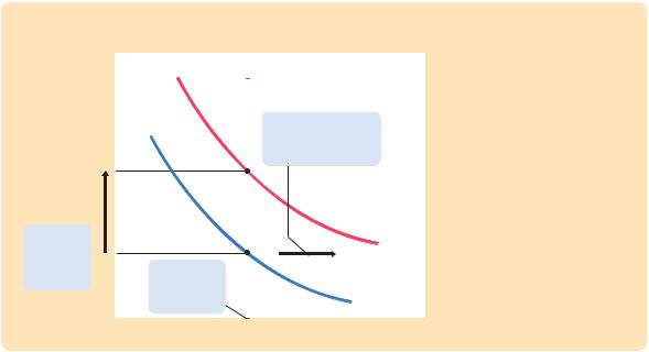
influence spending? To answer this question, we once again need to think about the international flow of capital and its implications for the domestic economy.

The interest rate and the exchange rate are again the key variables. As soon as an increase in the money supply starts putting downward pressure on the domestic interest rate, capital flows out of the economy, as investors seek a higher return elsewhere. This capital outflow prevents the domestic interest rate from falling below the world interest rate r*. It also has another effect: because investing abroad requires converting domestic currency into foreign currency, the capital outflow increases the supply of the domestic currency in the market for foreigncurrency exchange, causing the domestic currency to depreciate in value. This depreciation makes domestic goods inexpensive relative to foreign goods, stimulating net exports and thus total income. Hence, in a small open economy, monetary policy influences income by altering the exchange rate rather than the interest rate.

Trade Policy

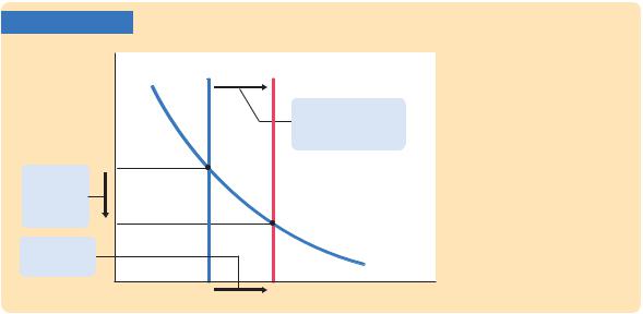
Suppose that the government reduces the demand for imported goods by imposing an import quota or a tariff. What happens to aggregate income and the exchange rate? How does the economy reach its new equilibrium?

Because net exports equal exports minus imports, a reduction in imports means an increase in net exports. That is, the net-exports schedule shifts to the right, as in Figure 12-6. This shift in the net-exports schedule increases planned expenditure and thus moves the IS* curve to the right. Because the LM* curve is vertical, the trade restriction raises the exchange rate but does not affect income.

The economic forces behind this transition are similar to the case of expansionary fiscal policy. Because net exports are a component of GDP, the rightward shift in the net-exports schedule, other things equal, puts upward pressure on income Y; an increase in Y, in turn, increases money demand and puts upward pressure on the interest rate r. Foreign capital quickly responds by flowing into the domestic economy, pushing the interest rate back to the world interest rate r* and causing the domestic currency to appreciate in value. Finally, the appreciation of the currency makes domestic goods more expensive relative to foreign goods, which decreases net exports NX and returns income Y to its initial level.

Often a stated goal of policies to restrict trade is to alter the trade balance NX. Yet, as we first saw in Chapter 5, such policies do not necessarily have that effect. The same conclusion holds in the Mundell–Fleming model under floating exchange rates. Recall that

NX(e) = Y − C(Y − T ) − I(r *) − G.

Because a trade restriction does not affect income, consumption, investment, or government purchases, it does not affect the trade balance. Although the shift in the net-exports schedule tends to raise NX, the increase in the exchange rate reduces NX by the same amount. The overall effect is simply less trade. The domestic economy imports less than it did before the trade restriction, but it exports less as well.