258 | P A R T I V Business Cycle Theory: The Economy in the Short Run

These historical events raise a variety of related questions: What causes shortrun fluctuations? What model should we use to explain them? Can policymakers avoid recessions? If so, what policy levers should they use?

In Parts Two and Three of this book, we developed theories to explain how the economy behaves in the long run. Here, in Part Four, we see how economists explain short-run fluctuations. We begin in this chapter with three tasks. First, we examine the data that describe short-run economic fluctuations. Second, we discuss the key differences between how the economy behaves in the long run and how it behaves in the short run. Third, we introduce the model of aggregate supply and aggregate demand, which most economists use to explain short-run fluctuations. Developing this model in more detail will be our primary job in the chapters that follow.

Just as Egypt now controls the flooding of the Nile Valley with the Aswan Dam, modern society tries to control the business cycle with appropriate economic policies. The model we develop over the next several chapters shows how monetary and fiscal policies influence the business cycle. We will see how these policies can potentially stabilize the economy or, if poorly conducted, make the problem of economic instability even worse.

9-1 The Facts About the Business Cycle

Before thinking about the theory of business cycles, let’s look at some of the facts that describe short-run fluctuations in economic activity.

GDP and Its Components

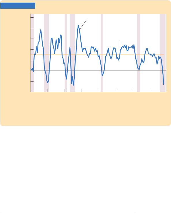
The economy’s gross domestic product measures total income and total expenditure in the economy. Because GDP is the broadest gauge of overall economic conditions, it is the natural place to start in analyzing the business cycle. Figure 9-1 shows the growth of real GDP from 1970 to early 2009. The horizontal line shows the average growth rate of 3 percent per year over this period. You can see that economic growth is not at all steady and that, occasionally, it turns negative.

The shaded areas in the figure indicate periods of recession. The official arbiter of when recessions begin and end is the National Bureau of Economic Research, a nonprofit economic research group. The NBER’s Business Cycle Dating Committee (of which the author of this book was once a member) chooses the starting date of each recession, called the business cycle peak, and the ending date, called the business cycle trough.

What determines whether a downturn in the economy is sufficiently severe to be deemed a recession? There is no simple answer. According to an old rule of thumb, a recession is a period of at least two consecutive quarters of declining real GDP. This rule, however, does not always hold. In the most recently revised data, for example, the recession of 2001 had two quarters of negative

260 | P A R T I V Business Cycle Theory: The Economy in the Short Run

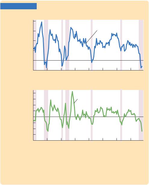
Growth in Consumption and Investment When the economy heads into a recession, growth in real consumption and investment spending both decline. Investment spending, shown in panel (b), is considerably more volatile than consumption spending, shown in panel (a). The shaded areas represent periods of recession.

Source: U.S. Department of Commerce.

Unemployment and Okun’s Law

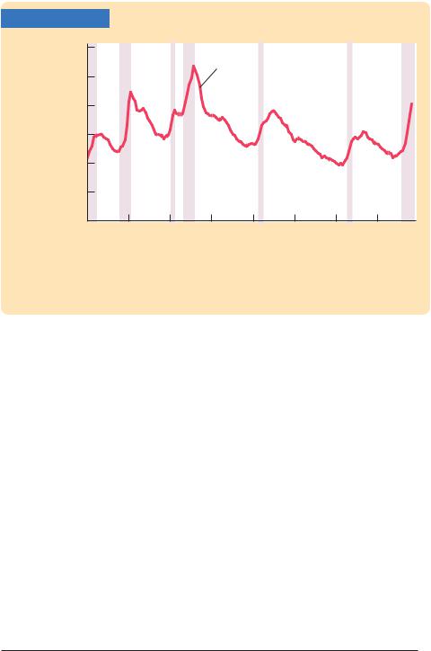
The business cycle is apparent not only in data from the national income accounts but also in data that describe conditions in the labor market. Figure 9-3 shows the unemployment rate from 1970 to early 2009, again with the shaded areas representing periods of recession. You can see that unemployment rises in each recession. Other labor-market measures tell a similar story. For example, job vacancies, as measured by the number of help-wanted ads in

Unemployment The unemployment rate rises significantly during periods of recession, shown here by the shaded areas.

Source: U.S. Department of Labor.

newspapers, decline during recessions. Put simply, during an economic downturn, jobs are harder to find.

What relationship should we expect to find between unemployment and real GDP? Because employed workers help to produce goods and services and unemployed workers do not, increases in the unemployment rate should be associated with decreases in real GDP. This negative relationship between unemployment and GDP is called Okun’s law, after Arthur Okun, the economist who first studied it.2

Figure 9-4 uses annual data for the United States to illustrate Okun’s law. In this scatterplot, each point represents the data for one year. The horizontal axis represents the change in the unemployment rate from the previous year, and the vertical axis represents the percentage change in GDP. This figure shows clearly that year-to-year changes in the unemployment rate are closely associated with year-to-year changes in real GDP.

We can be more precise about the magnitude of the Okun’s law relationship. The line drawn through the scatter of points tells us that

Percentage Change in Real GDP

= 3% − 2 × Change in the Unemployment Rate.

2 Arthur M. Okun, “Potential GNP: Its Measurement and Significance,’’ in Proceedings of the Business and Economics Statistics Section, American Statistical Association (Washington, D.C.: American Statistical Association, 1962): 98–103; reprinted in Arthur M. Okun, Economics for Policymaking (Cambridge, MA: MIT Press, 1983), 145–158.

262 | P A R T I V Business Cycle Theory: The Economy in the Short Run

FIGURE 9-4

Percentage change in real GDP

10

81951

Change in unemployment rate

Okun’s Law This figure is a scatterplot of the change in the unemployment rate on the horizontal axis and the percentage change in real GDP on the vertical axis, using data on the U.S economy. Each point represents one year. The negative correlation between these variables shows that increases in unemployment tend to be associated with lower-than-normal growth in real GDP.

Sources: U.S. Department of Commerce, U.S. Department of Labor.

If the unemployment rate remains the same, real GDP grows by about 3 percent; this normal growth in the production of goods and services is due to growth in the labor force, capital accumulation, and technological progress. In addition, for every percentage point the unemployment rate rises, real GDP growth typically falls by 2 percent. Hence, if the unemployment rate rises from 5 to 7 percent, then real GDP growth would be

Percentage Change in Real GDP = 3% − 2 × (7% − 5%)

= −1%.

In this case, Okun’s law says that GDP would fall by 1 percent, indicating that the economy is in a recession.

Okun’s law is a reminder that the forces that govern the short-run business cycle are very different from those that shape long-run economic growth. As we saw in Chapters 7 and 8, long-run growth in GDP is determined primarily by technological progress. The long-run trend leading to higher standards of living from generation to generation is not associated with any long-run trend in the rate of unemployment. By contrast, short-run movements in GDP are highly