C H A P T E R 1 8 Investment | 539

potentially profitable investment projects. Such an increase in financing constraints is sometimes called a credit crunch.

We can use the IS–LM model to interpret the short-run effects of a credit crunch. When some would-be investors are denied credit, the demand for investment goods falls at every interest rate. The result is a contractionary shift in the IS curve. This reduces aggregate demand, production, and employment.

The long-run effects of a credit crunch are best understood from the perspective of growth theory, with its emphasis on capital accumulation as a source of growth. When a credit crunch prevents some firms from investing, the financial markets fail to allocate national saving to its best use. Less productive investment projects may take the place of more productive projects, reducing the economy’s potential for producing goods and services.

Because of these effects, policymakers at the Fed and other parts of government are always trying to monitor the health of the nation’s banking system. Their goal is to avert banking crises and credit crunches and, when they do occur, to respond quickly to minimize the resulting disruption to the economy.

That job is not easy, as the financial crisis and economic downturn of 2008–2009 illustrates. In this case, as we discussed in Chapter 11, many banks had made large bets on the housing markets through their purchases of mortgage-backed securities. When those bets turned bad, many banks found themselves insolvent or nearly so, and bank loans became hard to come by. Bank regulators at the Federal Reserve and other government agencies, like many of the bankers themselves, were caught off guard by the magnitude of the losses and the resulting precariousness of the banking system. What kind of regulatory changes will be needed to try to reduce the likelihood of future banking crises remains a topic of active debate.

18-2 Residential Investment

In this section we consider the determinants of residential investment. We begin by presenting a simple model of the housing market. Residential investment includes the purchase of new housing both by people who plan to live in it themselves and by landlords who plan to rent it to others. To keep things simple, however, it is useful to imagine that all housing is owner-occupied.

The Stock Equilibrium and the Flow Supply

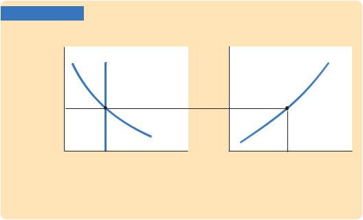
There are two parts to the model. First, the market for the existing stock of houses determines the equilibrium housing price. Second, the housing price determines the flow of residential investment.

Panel (a) of Figure 18-5 shows how the relative price of housing PH/P is determined by the supply and demand for the existing stock of houses. At any point in time, the supply of houses is fixed. We represent this stock with a vertical supply curve. The demand curve for houses slopes downward, because high prices cause people to live in smaller houses, to share residences, or sometimes even to become homeless. The price of housing adjusts to equilibrate supply and demand.

540 | P A R T V I More on the Microeconomics Behind Macroeconomics

FIGURE 18-5

Demand

The Determination of Residential Investment The relative price of housing adjusts to equilibrate supply and demand for the existing stock of housing capital. The relative price then determines residential investment, the flow of new housing that construction firms build.

Panel (b) of Figure 18-5 shows how the relative price of housing determines the supply of new houses. Construction firms buy materials and hire labor to build houses and then sell the houses at the market price. Their costs depend on the overall price level P (which reflects the cost of wood, bricks, plaster, etc.), and their revenue depends on the price of houses PH. The higher the relative price of housing, the greater the incentive to build houses and the more houses are built. The flow of new houses—residential investment—therefore depends on the equilibrium price set in the market for existing houses.

This model of residential investment is similar to the q theory of business fixed investment. According to the q theory, business fixed investment depends on the market price of installed capital relative to its replacement cost; this relative price, in turn, depends on the expected profits from owning installed capital. According to this model of the housing market, residential investment depends on the relative price of housing. The relative price of housing, in turn, depends on the demand for housing, which depends on the imputed rent that individuals expect to receive from their housing. Hence, the relative price of housing plays much the same role for residential investment as Tobin’s q does for business fixed investment.

Changes in Housing Demand

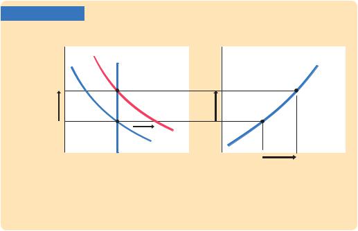
When the demand for housing shifts, the equilibrium price of housing changes, and this change in turn affects residential investment. The demand curve for housing can shift for various reasons. An economic boom raises national income and therefore the demand for housing. A large increase in the population, perhaps because of immigration, also raises the demand for housing. Panel (a) of Figure 18-6 shows that an expansionary shift in demand raises the equilibrium

C H A P T E R 1 8 Investment | 541

FIGURE 18-6

An Increase in Housing Demand An increase in housing demand, perhaps attributable to a fall in the interest rate, raises housing prices and residential investment.

price. Panel (b) shows that the increase in the housing price increases residential investment.

One important determinant of housing demand is the real interest rate. Many people take out loans—mortgages—to buy their homes; the interest rate is the cost of the loan. Even the few people who do not have to borrow to purchase a home will respond to the interest rate, because the interest rate is the opportunity cost of holding their wealth in housing rather than putting it in a bank. A reduction in the interest rate therefore raises housing demand, housing prices, and residential investment.

Another important determinant of housing demand is credit availability. When it is easy to get a loan, more households buy their own homes, and they buy larger ones than they otherwise might, thus increasing the demand for housing. When credit conditions become tight, fewer people buy their own homes or trade up to larger ones, and the demand for housing falls.

An example of this phenomenon occurred during the first decade of the 2000s. Early in this decade, interest rates were low, and mortgages were easy to come by. Many households with questionable credit histories—called subprime borrowers—were able to get mortgages with small down payments. Not surprisingly, the housing market boomed. Housing prices rose, and residential investment was strong. A few years later, however, it became clear that the situation had gotten out of hand, as many of these subprime borrowers could not keep up with their mortgage payments. When interest rates rose and credit conditions tightened, housing demand and housing prices started to fall. Figure 18-7 illustrates the movement of housing prices and housing starts during this period. When the housing market turned down in 2007 and 2008, the result was a significant downturn in the overall economy, which is discussed in a Case Study in Chapter 11.