How Monetary Policy Shifts the LM Curve

306 | P A R T I V Business Cycle Theory: The Economy in the Short Run

FIGURE 10-12

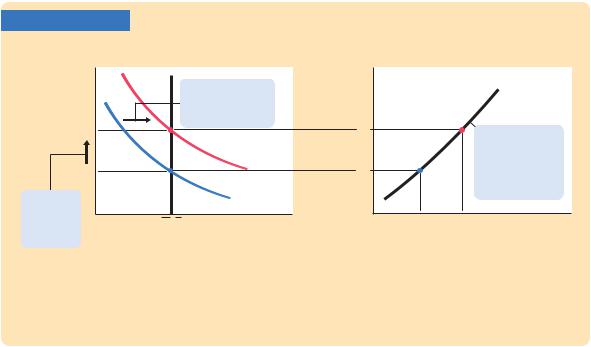
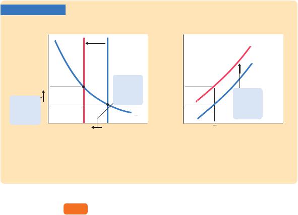
A Reduction in the Money Supply Shifts the LM Curve Upward Panel (a)

−

shows that for any given level of income Y, a reduction in the money supply raises the interest rate that equilibrates the money market. Therefore, the LM curve in panel (b) shifts upward.

10-3 Conclusion:

The Short-Run Equilibrium

We now have all the pieces of the IS –LM model. The two equations of this model are

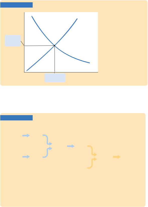
The model takes fiscal policy G and T, monetary policy M, and the price level P as exogenous. Given these exogenous variables, the IS curve provides the combinations of r and Y that satisfy the equation representing the goods market, and the LM curve provides the combinations of r and Y that satisfy the equation representing the money market. These two curves are shown together in Figure 10-13.

The equilibrium of the economy is the point at which the IS curve and the LM curve cross. This point gives the interest rate r and the level of income Y that satisfy conditions for equilibrium in both the goods market and the money market. In other words, at this intersection, actual expenditure equals planned expenditure, and the demand for real money balances equals the supply.

As we conclude this chapter, let’s recall that our ultimate goal in developing the IS –LM model is to analyze short-run fluctuations in economic activity. Figure 10-14 illustrates how the different pieces of our theory fit together.

308 | P A R T I V Business Cycle Theory: The Economy in the Short Run

the aggregate demand curve. The aggregate demand curve, in turn, is a piece of the model of aggregate supply and aggregate demand, which economists use to explain the short-run effects of policy changes and other events on national income.

Summary

1.The Keynesian cross is a basic model of income determination. It takes fiscal policy and planned investment as exogenous and then shows that there is one level of national income at which actual expenditure equals planned expenditure. It shows that changes in fiscal policy have a multiplied impact on income.

2.Once we allow planned investment to depend on the interest rate, the Keynesian cross yields a relationship between the interest rate

and national income. A higher interest rate lowers planned investment, and this in turn lowers national income. The downward-sloping IS curve summarizes this negative relationship between the interest rate and income.

3.The theory of liquidity preference is a basic model of the determination of the interest rate. It takes the money supply and the price level as exogenous and assumes that the interest rate adjusts to equilibrate the supply and demand for real money balances. The theory implies that increases in the money supply lower the interest rate.

4.Once we allow the demand for real money balances to depend on national income, the theory of liquidity preference yields a relationship between income and the interest rate. A higher level of income raises the demand for real money balances, and this in turn raises the

interest rate. The upward-sloping LM curve summarizes this positive relationship between income and the interest rate.

5.The IS –LM model combines the elements of the Keynesian cross and the elements of the theory of liquidity preference. The IS curve shows the points that satisfy equilibrium in the goods market, and the LM curve shows the points that satisfy equilibrium in the money market. The intersection of the IS and LM curves shows the interest rate and income that satisfy equilibrium in both markets for a given price level.

312 | P A R T I V Business Cycle Theory: The Economy in the Short Run

of this traumatic economic downturn. And, as we will see throughout this chapter, the model can also be used to shed light on more recent recessions, such as those that began in 2001 and 2008.

11-1 Explaining Fluctuations With the

IS–LM Model

The intersection of the IS curve and the LM curve determines the level of national income. When one of these curves shifts, the short-run equilibrium of the economy changes, and national income fluctuates. In this section we examine how changes in policy and shocks to the economy can cause these curves to shift.

How Fiscal Policy Shifts the IS Curve and

Changes the Short-Run Equilibrium

We begin by examining how changes in fiscal policy (government purchases and taxes) alter the economy’s short-run equilibrium. Recall that changes in fiscal policy influence planned expenditure and thereby shift the IS curve. The IS –LM model shows how these shifts in the IS curve affect income and the interest rate.

Changes in Government Purchases Consider an increase in government purchases of G. The government-purchases multiplier in the Keynesian cross tells us that this change in fiscal policy raises the level of income at any given interest rate by G/(1 − MPC). Therefore, as Figure 11-1 shows, the IS curve shifts to the right

FIGURE 11-1

C H A P T E R 1 1 Aggregate Demand II: Applying the IS-LM Model | 313

by this amount. The equilibrium of the economy moves from point A to point B. The increase in government purchases raises both income and the interest rate.

To understand fully what’s happening in Figure 11-1, it helps to keep in mind the building blocks for the IS –LM model from the preceding chapter—the Keynesian cross and the theory of liquidity preference. Here is the story. When the government increases its purchases of goods and services, the economy’s planned expenditure rises. The increase in planned expenditure stimulates the production of goods and services, which causes total income Y to rise. These effects should be familiar from the Keynesian cross.

Now consider the money market, as described by the theory of liquidity preference. Because the economy’s demand for money depends on income, the rise in total income increases the quantity of money demanded at every interest rate. The supply of money has not changed, however, so higher money demand causes the equilibrium interest rate r to rise.

The higher interest rate arising in the money market, in turn, has ramifications back in the goods market. When the interest rate rises, firms cut back on their investment plans. This fall in investment partially offsets the expansionary effect of the increase in government purchases. Thus, the increase in income in response to a fiscal expansion is smaller in the IS –LM model than it is in the Keynesian cross (where investment is assumed to be fixed). You can see this in Figure 11-1. The horizontal shift in the IS curve equals the rise in equilibrium income in the Keynesian cross. This amount is larger than the increase in equilibrium income here in the IS –LM model. The difference is explained by the crowding out of investment due to a higher interest rate.

Changes in Taxes In the IS –LM model, changes in taxes affect the economy much the same as changes in government purchases do, except that taxes affect expenditure through consumption. Consider, for instance, a decrease in taxes of T. The tax cut encourages consumers to spend more and, therefore, increases planned expenditure. The tax multiplier in the Keynesian cross tells us that this change in policy raises the level of income at any given interest rate by

T × MPC/(1 − MPC ). Therefore, as Figure 11-2 illustrates, the IS curve shifts to the right by this amount. The equilibrium of the economy moves from point A to point B. The tax cut raises both income and the interest rate. Once again, because the higher interest rate depresses investment, the increase in income is smaller in the IS –LM model than it is in the Keynesian cross.

How Monetary Policy Shifts the LM Curve

and Changes the Short-Run Equilibrium

We now examine the effects of monetary policy. Recall that a change in the money supply alters the interest rate that equilibrates the money market for any given level of income and, thus, shifts the LM curve. The IS –LM model shows how a shift in the LM curve affects income and the interest rate.

Consider an increase in the money supply. An increase in M leads to an increase in real money balances M/P, because the price level P is fixed in the short run. The theory of liquidity preference shows that for any given level of

C H A P T E R 1 1 Aggregate Demand II: Applying the IS-LM Model | 315

Reserve increases the supply of money, people have more money than they want to hold at the prevailing interest rate. As a result, they start depositing this extra money in banks or using it to buy bonds. The interest rate r then falls until people are willing to hold all the extra money that the Fed has created; this brings the money market to a new equilibrium. The lower interest rate, in turn, has ramifications for the goods market. A lower interest rate stimulates planned investment, which increases planned expenditure, production, and income Y.

Thus, the IS–LM model shows that monetary policy influences income by changing the interest rate. This conclusion sheds light on our analysis of monetary policy in Chapter 9. In that chapter we showed that in the short run, when prices are sticky, an expansion in the money supply raises income. But we did not discuss how a monetary expansion induces greater spending on goods and services—a process called the monetary transmission mechanism. The IS–LM model shows an important part of that mechanism: an increase in the money supply lowers the interest rate, which stimulates investment and thereby expands the demand for goods and services. The next chapter shows that in open economies, the exchange rate also has a role in the monetary transmission mechanism; for large economies such as that of the United States, however, the interest rate has the leading role.

The Interaction Between Monetary and Fiscal Policy

When analyzing any change in monetary or fiscal policy, it is important to keep in mind that the policymakers who control these policy tools are aware of what the other policymakers are doing. A change in one policy, therefore, may influence the other, and this interdependence may alter the impact of a policy change.

For example, suppose Congress raises taxes. What effect will this policy have on the economy? According to the IS –LM model, the answer depends on how the Fed responds to the tax increase.

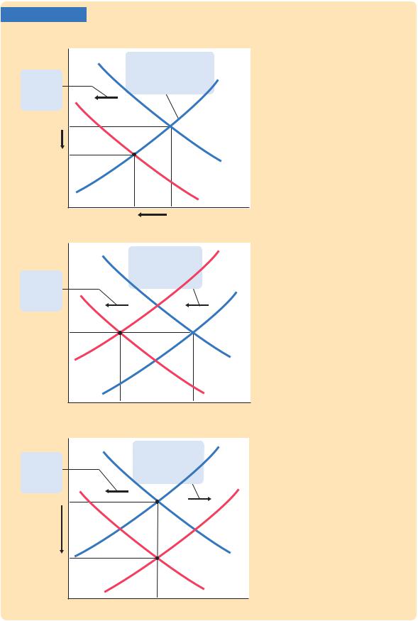
Figure 11-4 shows three of the many possible outcomes. In panel (a), the Fed holds the money supply constant. The tax increase shifts the IS curve to the left. Income falls (because higher taxes reduce consumer spending), and the interest rate falls (because lower income reduces the demand for money). The fall in income indicates that the tax hike causes a recession.

In panel (b), the Fed wants to hold the interest rate constant. In this case, when the tax increase shifts the IS curve to the left, the Fed must decrease the money supply to keep the interest rate at its original level. This fall in the money supply shifts the LM curve upward. The interest rate does not fall, but income falls by a larger amount than if the Fed had held the money supply constant. Whereas in panel (a) the lower interest rate stimulated investment and partially offset the contractionary effect of the tax hike, in panel (b) the Fed deepens the recession by keeping the interest rate high.

In panel (c), the Fed wants to prevent the tax increase from lowering income. It must, therefore, raise the money supply and shift the LM curve downward enough to offset the shift in the IS curve. In this case, the tax increase does not cause a recession, but it does cause a large fall in the interest rate. Although the level of income is not changed, the combination of a tax increase and a monetary expansion does change the allocation of the economy’s resources. The

C H A P T E R 1 1 Aggregate Demand II: Applying the IS-LM Model | 317

higher taxes depress consumption, while the lower interest rate stimulates investment. Income is not affected because these two effects exactly balance.

From this example we can see that the impact of a change in fiscal policy depends on the policy the Fed pursues—that is, on whether it holds the money supply, the interest rate, or the level of income constant. More generally, whenever analyzing a change in one policy, we must make an assumption about its effect on the other policy. The most appropriate assumption depends on the case at hand and the many political considerations that lie behind economic policymaking.

CASE STUDY

Policy Analysis With Macroeconometric Models

The IS–LM model shows how monetary and fiscal policy influence the equilibrium level of income. The predictions of the model, however, are qualitative, not quantitative. The IS–LM model shows that increases in government purchases raise GDP and that increases in taxes lower GDP. But when economists analyze specific policy proposals, they need to know not only the direction of the effect but also the size. For example, if Congress increases taxes by $100 billion and if monetary policy is not altered, how much will GDP fall? To answer this question, economists need to go beyond the graphical representation of the IS–LM model.

Macroeconometric models of the economy provide one way to evaluate policy proposals. A macroeconometric model is a model that describes the economy quantitatively, rather than just qualitatively. Many of these models are essentially more complicated and more realistic versions of our IS –LM model. The economists who build macroeconometric models use historical data to estimate parameters such as the marginal propensity to consume, the sensitivity of investment to the interest rate, and the sensitivity of money demand to the interest rate. Once a model is built, economists can simulate the effects of alternative policies with the help of a computer.

Table 11-1 shows the fiscal-policy multipliers implied by one widely used macroeconometric model, the Data Resources Incorporated (DRI) model, named for the economic forecasting firm that developed it. The multipliers are given for two assumptions about how the Fed might respond to changes in fiscal policy.

One assumption about monetary policy is that the Fed keeps the nominal interest rate constant. That is, when fiscal policy shifts the IS curve to the right or to the left, the Fed adjusts the money supply to shift the LM curve in the same direction. Because there is no crowding out of investment due to a changing interest rate, the fiscal-policy multipliers are similar to those from the Keynesian cross. The DRI model indicates that, in this case, the government-purchases multiplier is 1.93, and the tax multiplier is −1.19. That is, a $100 billion increase in government purchases raises GDP by $193 billion, and a $100 billion increase in taxes lowers GDP by $119 billion.

The second assumption about monetary policy is that the Fed keeps the money supply constant so that the LM curve does not shift. In this case, the interest rate rises, and investment is crowded out, so the multipliers are much smaller. The gov- ernment-purchases multiplier is only 0.60, and the tax multiplier is only −0.26.