Inflation differential

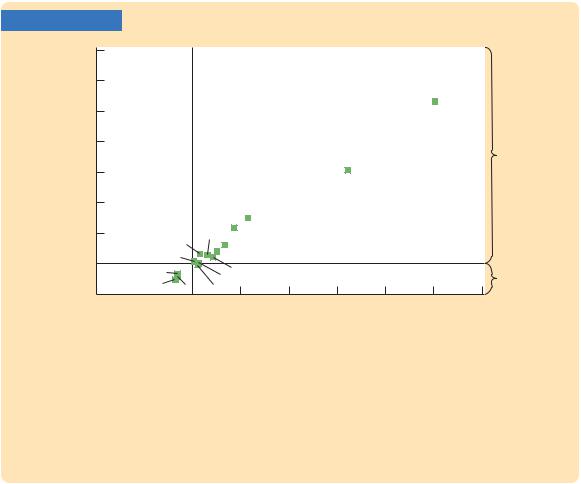
Inflation Differentials and the Exchange Rate This scatterplot shows the relationship between inflation and the nominal exchange rate. The horizontal axis shows the country’s average inflation rate minus the U.S. average inflation rate over the period 1972–2007. The vertical axis is the average percentage change in the country’s exchange rate (per U.S. dollar) over that period. This figure shows that countries with relatively high inflation tend to have depreciating currencies and that countries with relatively low inflation tend to have appreciating currencies.

Source: International Monetary Fund.

did. But, as Figure 5-13 shows, inflation in Switzerland has been lower than inflation in the United States. This means that the value of the franc has fallen less than the value of the dollar. Therefore, the number of Swiss francs you can buy with a U.S. dollar has been falling over time. ■

The Special Case of Purchasing-Power Parity

A famous hypothesis in economics, called the law of one price, states that the same good cannot sell for different prices in different locations at the same time. If a bushel of wheat sold for less in New York than in Chicago, it would be profitable to buy wheat in New York and then sell it in Chicago. This profit opportunity would become quickly apparent to astute arbitrageurs—people who specialize in “buying low” in one market and “selling high” in another. As the arbitrageurs took advantage of this opportunity, they would increase the demand for wheat in New York and increase the supply of wheat in Chicago. Their

C H A P T E R 5 The Open Economy | 149

exchange rate of 10.2. Yet the theory’s predictions are far from exact and, in many cases, are off by 30 percent or more. Hence, although the theory of pur- chasing-power parity provides a rough guide to the level of exchange rates, it does not explain exchange rates completely. ■

5-3 Conclusion: The United States

as a Large Open Economy

In this chapter we have seen how a small open economy works. We have examined the determinants of the international flow of funds for capital accumulation and the international flow of goods and services. We have also examined the determinants of a country’s real and nominal exchange rates. Our analysis shows how various policies—monetary policies, fiscal policies, and trade policies— affect the trade balance and the exchange rate.

The economy we have studied is “small’’ in the sense that its interest rate is fixed by world financial markets. That is, we have assumed that this economy does not affect the world interest rate and that the economy can borrow and lend at the world interest rate in unlimited amounts. This assumption contrasts with the assumption we made when we studied the closed economy in Chapter 3. In the closed economy, the domestic interest rate equilibrates domestic saving and domestic investment, implying that policies that influence saving or investment alter the equilibrium interest rate.

Which of these analyses should we apply to an economy such as that of the United States? The answer is a little of both. The United States is neither so large nor so isolated that it is immune to developments occurring abroad. The large trade deficits of the 1980s, 1990s, and 2000s show the importance of international financial markets for funding U.S. investment. Hence, the closed-economy analysis of Chapter 3 cannot by itself fully explain the impact of policies on the U.S. economy.

Yet the U.S. economy is not so small and so open that the analysis of this chapter applies perfectly either. First, the United States is large enough that it can influence world financial markets. For example, large U.S. budget deficits were often blamed for the high real interest rates that prevailed throughout the world in the 1980s. Second, capital may not be perfectly mobile across countries. If individuals prefer holding their wealth in domestic rather than foreign assets, funds for capital accumulation will not flow freely to equate interest rates in all countries. For these two reasons, we cannot directly apply our model of the small open economy to the United States.

When analyzing policy for a country such as the United States, we need to combine the closed-economy logic of Chapter 3 and the small-open-economy logic of this chapter. The appendix to this chapter builds a model of an economy between these two extremes. In this intermediate case, there is international borrowing and lending, but the interest rate is not fixed by world financial markets. Instead, the more the economy borrows from abroad, the higher the interest rate it must offer foreign investors. The results, not surprisingly, are a mixture of the two polar cases we have already examined.

150 | P A R T I I Classical Theory: The Economy in the Long Run

Consider, for example, a reduction in national saving due to a fiscal expansion. As in the closed economy, this policy raises the real interest rate and crowds out domestic investment. As in the small open economy, it also reduces the net capital outflow, leading to a trade deficit and an appreciation of the exchange rate. Hence, although the model of the small open economy examined here does not precisely describe an economy such as that of the United States, it does provide approximately the right answer to how policies affect the trade balance and the exchange rate.

Summary

1.Net exports are the difference between exports and imports. They are equal to the difference between what we produce and what we demand for consumption, investment, and government purchases.

2.The net capital outflow is the excess of domestic saving over domestic investment. The trade balance is the amount received for our net exports of goods and services. The national income accounts identity shows that the net capital outflow always equals the trade balance.

3.The impact of any policy on the trade balance can be determined by examining its impact on saving and investment. Policies that raise saving or lower investment lead to a trade surplus, and policies that lower saving or raise investment lead to a trade deficit.

4.The nominal exchange rate is the rate at which people trade the currency of one country for the currency of another country. The real exchange rate is the rate at which people trade the goods produced by the two countries. The real exchange rate equals the nominal exchange rate multiplied by the ratio of the price levels in the two countries.

5.Because the real exchange rate is the price of domestic goods relative to foreign goods, an appreciation of the real exchange rate tends to reduce net exports. The equilibrium real exchange rate is the rate at which the quantity of net exports demanded equals the net capital outflow.

6.The nominal exchange rate is determined by the real exchange rate and the price levels in the two countries. Other things equal, a high rate of inflation leads to a depreciating currency.

K E Y C O N C E P T S