

- •About the author
- •Brief Contents
- •Contents
- •Preface
- •This Book’s Approach
- •What’s New in the Seventh Edition?
- •The Arrangement of Topics
- •Part One, Introduction
- •Part Two, Classical Theory: The Economy in the Long Run
- •Part Three, Growth Theory: The Economy in the Very Long Run
- •Part Four, Business Cycle Theory: The Economy in the Short Run
- •Part Five, Macroeconomic Policy Debates
- •Part Six, More on the Microeconomics Behind Macroeconomics
- •Epilogue
- •Alternative Routes Through the Text
- •Learning Tools
- •Case Studies
- •FYI Boxes
- •Graphs
- •Mathematical Notes
- •Chapter Summaries
- •Key Concepts
- •Questions for Review
- •Problems and Applications
- •Chapter Appendices
- •Glossary
- •Translations
- •Acknowledgments
- •Supplements and Media
- •For Instructors
- •Instructor’s Resources
- •Solutions Manual
- •Test Bank
- •PowerPoint Slides
- •For Students
- •Student Guide and Workbook
- •Online Offerings
- •EconPortal, Available Spring 2010
- •eBook
- •WebCT
- •BlackBoard
- •Additional Offerings
- •i-clicker
- •The Wall Street Journal Edition
- •Financial Times Edition
- •Dismal Scientist
- •1-1: What Macroeconomists Study
- •1-2: How Economists Think
- •Theory as Model Building
- •The Use of Multiple Models
- •Prices: Flexible Versus Sticky
- •Microeconomic Thinking and Macroeconomic Models
- •1-3: How This Book Proceeds
- •Income, Expenditure, and the Circular Flow
- •Rules for Computing GDP
- •Real GDP Versus Nominal GDP
- •The GDP Deflator
- •Chain-Weighted Measures of Real GDP
- •The Components of Expenditure
- •Other Measures of Income
- •Seasonal Adjustment
- •The Price of a Basket of Goods
- •The CPI Versus the GDP Deflator
- •The Household Survey
- •The Establishment Survey
- •The Factors of Production
- •The Production Function
- •The Supply of Goods and Services
- •3-2: How Is National Income Distributed to the Factors of Production?
- •Factor Prices
- •The Decisions Facing the Competitive Firm
- •The Firm’s Demand for Factors
- •The Division of National Income
- •The Cobb–Douglas Production Function
- •Consumption
- •Investment
- •Government Purchases
- •Changes in Saving: The Effects of Fiscal Policy
- •Changes in Investment Demand
- •3-5: Conclusion
- •4-1: What Is Money?
- •The Functions of Money
- •The Types of Money
- •The Development of Fiat Money
- •How the Quantity of Money Is Controlled
- •How the Quantity of Money Is Measured
- •4-2: The Quantity Theory of Money
- •Transactions and the Quantity Equation
- •From Transactions to Income
- •The Assumption of Constant Velocity
- •Money, Prices, and Inflation
- •4-4: Inflation and Interest Rates
- •Two Interest Rates: Real and Nominal
- •The Fisher Effect
- •Two Real Interest Rates: Ex Ante and Ex Post
- •The Cost of Holding Money
- •Future Money and Current Prices
- •4-6: The Social Costs of Inflation
- •The Layman’s View and the Classical Response
- •The Costs of Expected Inflation
- •The Costs of Unexpected Inflation
- •One Benefit of Inflation
- •4-7: Hyperinflation
- •The Costs of Hyperinflation
- •The Causes of Hyperinflation
- •4-8: Conclusion: The Classical Dichotomy
- •The Role of Net Exports
- •International Capital Flows and the Trade Balance
- •International Flows of Goods and Capital: An Example
- •Capital Mobility and the World Interest Rate
- •Why Assume a Small Open Economy?
- •The Model
- •How Policies Influence the Trade Balance
- •Evaluating Economic Policy
- •Nominal and Real Exchange Rates
- •The Real Exchange Rate and the Trade Balance
- •The Determinants of the Real Exchange Rate
- •How Policies Influence the Real Exchange Rate
- •The Effects of Trade Policies
- •The Special Case of Purchasing-Power Parity
- •Net Capital Outflow
- •The Model
- •Policies in the Large Open Economy
- •Conclusion
- •Causes of Frictional Unemployment
- •Public Policy and Frictional Unemployment
- •Minimum-Wage Laws
- •Unions and Collective Bargaining
- •Efficiency Wages
- •The Duration of Unemployment
- •Trends in Unemployment
- •Transitions Into and Out of the Labor Force
- •6-5: Labor-Market Experience: Europe
- •The Rise in European Unemployment
- •Unemployment Variation Within Europe
- •The Rise of European Leisure
- •6-6: Conclusion
- •7-1: The Accumulation of Capital
- •The Supply and Demand for Goods
- •Growth in the Capital Stock and the Steady State
- •Approaching the Steady State: A Numerical Example
- •How Saving Affects Growth
- •7-2: The Golden Rule Level of Capital
- •Comparing Steady States
- •The Transition to the Golden Rule Steady State
- •7-3: Population Growth
- •The Steady State With Population Growth
- •The Effects of Population Growth
- •Alternative Perspectives on Population Growth
- •7-4: Conclusion
- •The Efficiency of Labor
- •The Steady State With Technological Progress
- •The Effects of Technological Progress
- •Balanced Growth
- •Convergence
- •Factor Accumulation Versus Production Efficiency
- •8-3: Policies to Promote Growth
- •Evaluating the Rate of Saving
- •Changing the Rate of Saving
- •Allocating the Economy’s Investment
- •Establishing the Right Institutions
- •Encouraging Technological Progress
- •The Basic Model
- •A Two-Sector Model
- •The Microeconomics of Research and Development
- •The Process of Creative Destruction
- •8-5: Conclusion
- •Increases in the Factors of Production
- •Technological Progress
- •The Sources of Growth in the United States
- •The Solow Residual in the Short Run
- •9-1: The Facts About the Business Cycle
- •GDP and Its Components
- •Unemployment and Okun’s Law
- •Leading Economic Indicators
- •9-2: Time Horizons in Macroeconomics
- •How the Short Run and Long Run Differ
- •9-3: Aggregate Demand
- •The Quantity Equation as Aggregate Demand
- •Why the Aggregate Demand Curve Slopes Downward
- •Shifts in the Aggregate Demand Curve
- •9-4: Aggregate Supply
- •The Long Run: The Vertical Aggregate Supply Curve
- •From the Short Run to the Long Run
- •9-5: Stabilization Policy
- •Shocks to Aggregate Demand
- •Shocks to Aggregate Supply
- •10-1: The Goods Market and the IS Curve
- •The Keynesian Cross
- •The Interest Rate, Investment, and the IS Curve
- •How Fiscal Policy Shifts the IS Curve
- •10-2: The Money Market and the LM Curve
- •The Theory of Liquidity Preference
- •Income, Money Demand, and the LM Curve
- •How Monetary Policy Shifts the LM Curve
- •Shocks in the IS–LM Model
- •From the IS–LM Model to the Aggregate Demand Curve
- •The IS–LM Model in the Short Run and Long Run
- •11-3: The Great Depression
- •The Spending Hypothesis: Shocks to the IS Curve
- •The Money Hypothesis: A Shock to the LM Curve
- •Could the Depression Happen Again?
- •11-4: Conclusion
- •12-1: The Mundell–Fleming Model
- •The Goods Market and the IS* Curve
- •The Money Market and the LM* Curve
- •Putting the Pieces Together
- •Fiscal Policy
- •Monetary Policy
- •Trade Policy
- •How a Fixed-Exchange-Rate System Works
- •Fiscal Policy
- •Monetary Policy
- •Trade Policy
- •Policy in the Mundell–Fleming Model: A Summary
- •12-4: Interest Rate Differentials
- •Country Risk and Exchange-Rate Expectations
- •Differentials in the Mundell–Fleming Model
- •Pros and Cons of Different Exchange-Rate Systems
- •The Impossible Trinity
- •12-6: From the Short Run to the Long Run: The Mundell–Fleming Model With a Changing Price Level
- •12-7: A Concluding Reminder
- •Fiscal Policy
- •Monetary Policy
- •A Rule of Thumb
- •The Sticky-Price Model
- •Implications
- •Adaptive Expectations and Inflation Inertia
- •Two Causes of Rising and Falling Inflation
- •Disinflation and the Sacrifice Ratio
- •13-3: Conclusion
- •14-1: Elements of the Model
- •Output: The Demand for Goods and Services
- •The Real Interest Rate: The Fisher Equation
- •Inflation: The Phillips Curve
- •Expected Inflation: Adaptive Expectations
- •The Nominal Interest Rate: The Monetary-Policy Rule
- •14-2: Solving the Model
- •The Long-Run Equilibrium
- •The Dynamic Aggregate Supply Curve
- •The Dynamic Aggregate Demand Curve
- •The Short-Run Equilibrium
- •14-3: Using the Model
- •Long-Run Growth
- •A Shock to Aggregate Supply
- •A Shock to Aggregate Demand
- •A Shift in Monetary Policy
- •The Taylor Principle
- •14-5: Conclusion: Toward DSGE Models
- •15-1: Should Policy Be Active or Passive?
- •Lags in the Implementation and Effects of Policies
- •The Difficult Job of Economic Forecasting
- •Ignorance, Expectations, and the Lucas Critique
- •The Historical Record
- •Distrust of Policymakers and the Political Process
- •The Time Inconsistency of Discretionary Policy
- •Rules for Monetary Policy
- •16-1: The Size of the Government Debt
- •16-2: Problems in Measurement
- •Measurement Problem 1: Inflation
- •Measurement Problem 2: Capital Assets
- •Measurement Problem 3: Uncounted Liabilities
- •Measurement Problem 4: The Business Cycle
- •Summing Up
- •The Basic Logic of Ricardian Equivalence
- •Consumers and Future Taxes
- •Making a Choice
- •16-5: Other Perspectives on Government Debt
- •Balanced Budgets Versus Optimal Fiscal Policy
- •Fiscal Effects on Monetary Policy
- •Debt and the Political Process
- •International Dimensions
- •16-6: Conclusion
- •Keynes’s Conjectures
- •The Early Empirical Successes
- •The Intertemporal Budget Constraint
- •Consumer Preferences
- •Optimization
- •How Changes in Income Affect Consumption
- •Constraints on Borrowing
- •The Hypothesis
- •Implications
- •The Hypothesis
- •Implications
- •The Hypothesis
- •Implications
- •17-7: Conclusion
- •18-1: Business Fixed Investment
- •The Rental Price of Capital
- •The Cost of Capital
- •The Determinants of Investment
- •Taxes and Investment
- •The Stock Market and Tobin’s q
- •Financing Constraints
- •Banking Crises and Credit Crunches
- •18-2: Residential Investment
- •The Stock Equilibrium and the Flow Supply
- •Changes in Housing Demand
- •18-3: Inventory Investment
- •Reasons for Holding Inventories
- •18-4: Conclusion
- •19-1: Money Supply
- •100-Percent-Reserve Banking
- •Fractional-Reserve Banking
- •A Model of the Money Supply
- •The Three Instruments of Monetary Policy
- •Bank Capital, Leverage, and Capital Requirements
- •19-2: Money Demand
- •Portfolio Theories of Money Demand
- •Transactions Theories of Money Demand
- •The Baumol–Tobin Model of Cash Management
- •19-3 Conclusion
- •Lesson 2: In the short run, aggregate demand influences the amount of goods and services that a country produces.
- •Question 1: How should policymakers try to promote growth in the economy’s natural level of output?
- •Question 2: Should policymakers try to stabilize the economy?
- •Question 3: How costly is inflation, and how costly is reducing inflation?
- •Question 4: How big a problem are government budget deficits?
- •Conclusion
- •Glossary
- •Index

C H A P T E R 1 4 A Dynamic Model of Aggregate Demand and Aggregate Supply | 417
14-2 Solving the Model
We have now looked at each of the pieces of the dynamic AD –AS model. To summarize, here are the five equations that make up the model:
− |
− r) + et |
|
Yt = Y t − a (rt |
The Demand for Goods and Services |
|
rt = it − Et pt +1 |
− |
The Fisher Equation |
pt = Et −1pt + f(Yt − Yt ) + ut |
The Phillips Curve |
|
Et pt +1 = pt |
− |
Adaptive Expectations |
it = pt + r + vp(pt – p*t ) + vY(Yt − Yt) |
The Monetary-Policy Rule |
|
These five equations determine the paths of the model’s five endogenous variables: output Yt, the real interest rate rt, inflation pt, expected inflation Et pt +1, and the nominal interest rate it.
Table 14-1 lists all the variables and parameters in the model. In any period, the five endogenous variables are influenced by the four exogenous variables in
TA B L E 14-1
The Variables and Parameters in the Dynamic AD–AS Model
Endogenous Variables
Yt
pt
rt it
Etpt +1
Exogenous Variables
−
Yt
p*
t
et ut
Predetermined Variable
pt −1
Parameters
a
r
f
vp vY
Output
Inflation
Real interest rate
Nominal interest rate
Expected inflation
Natural level of output
Central bank’s target for inflation
Shock to the demand for goods and services Shock to the Phillips curve (supply shock)
Previous period’s inflation
The responsiveness of the demand for goods and services to the real interest rate
The natural rate of interest
The responsiveness of inflation to output in the Phillips curve
The responsiveness of the nominal interest rate to inflation in the monetary-policy rule
The responsiveness of the nominal interest rate to output in the monetary-policy rule
418 | P A R T I V Business Cycle Theory: The Economy in the Short Run
the equations as well as the previous period’s inflation rate. Lagged inflation pt −1 is called a predetermined variable. That is, it is a variable that was endogenous in the past but, because it is fixed by the time when we arrive in period t, is essentially exogenous for the purposes of finding the current equilibrium.
We are almost ready to put these pieces together to see how various shocks to the economy influence the paths of these variables over time. Before doing so, however, we need to establish the starting point for our analysis: the economy’s long-run equilibrium.
The Long-Run Equilibrium
The long-run equilibrium represents the normal state around which the economy fluctuates. It occurs when there are no shocks (et = ut = 0) and inflation has
stabilized (pt = pt −1).
Straightforward algebra applied to the above five equations can be used to verify these long-run values:
= −
Yt Yt. rt = r.
p = p*.
t t
E p + = p*.
t t 1 t
i = r + p*.
t t
In words, the long-run equilibrium is described as follows: output and the real interest rate are at their natural values, inflation and expected inflation are at the target rate of inflation, and the nominal interest rate equals the natural rate of interest plus target inflation.
The long-run equilibrium of this model reflects two related principles: the classical dichotomy and monetary neutrality. Recall that the classical dichotomy is the separation of real from nominal variables, and monetary neutrality is the property according to which monetary policy does not influence real variables.
The equations immediately above show that the central bank’s inflation target p*
t
influences only inflation pt, expected inflation Et pt+1, and the nominal interest rate it. If the central bank raises its inflation target, then inflation, expected inflation, and the nominal interest rate all increase by the same amount. The real variables—output Yt and the real interest rate rt—do not depend on monetary policy. In these ways, the long-run equilibrium of the dynamic AD –AS model mirrors the classical models we examined in Chapters 3 to 8.
The Dynamic Aggregate Supply Curve
To study the behavior of this economy in the short run, it is useful to analyze the model graphically. Because graphs have two axes, we need to focus on two variables. We will use output Yt and inflation pt as the variables on the two axes because these
C H A P T E R 1 4 A Dynamic Model of Aggregate Demand and Aggregate Supply | 419
are the variables of central interest. As in the conventional AD–AS model, output will be on the horizontal axis. But because the price level has now faded into the background, the vertical axis in our graphs will now represent the inflation rate.
To generate this graph, we need two equations that summarize the relationships between output Yt and inflation pt. These equations are derived from the five equations of the model we have already seen. To isolate the relationships between Yt and pt, however, we need to use a bit of algebra to eliminate the other three endogenous variables (rt, it, and Et −1pt ).
The first relationship between output and inflation comes almost directly from the Phillips curve equation. We can get rid of the one endogenous variable in the equation (Et −1pt) by using the expectations equation (Et −1pt = pt −1) to substitute past inflation pt −1 for expected inflation Et −1pt. With this substitution, the equation for the Phillips curve becomes
|
|
|
− |
|
|
pt = pt −1 + f(Yt − Yt) + ut. |
(DAS ) |
||
This equation relates inflation |
pt |
and output Y for given values of two exoge- |
||
− |
|
t |
|
|
nous variables (Yt |
and ut) and a predetermined variable (pt −1). |
|||
Figure 14-2 graphs the relationship between inflation |
pt and output Yt |
|||
described by this |
equation. We |
call this upward-sloping |
curve the dynamic |
|
aggregate supply curve, or DAS. The dynamic aggregate supply curve is similar to the aggregate supply curve we saw in Chapter 13, except that inflation rather than the price level is on the vertical axis. The DAS curve shows how inflation is related to output in the short run. Its upward slope reflects the Phillips curve: Other things equal, high levels of economic activity are associated with high inflation.
The DAS curve is drawn for given values of past inflation |
pt −1 |
, the natural |
− |
|
level of output Yt, and the supply shock ut. If any one of these three variables changes, the DAS curve shifts. One of our tasks ahead is to trace out the implications of such shifts. But first, we need another curve.
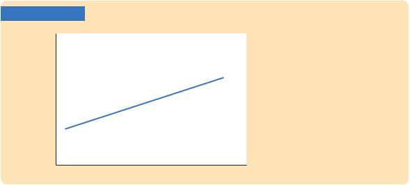
FIGURE 14-2 |
Inflation, p |
Dynamic aggregate |
supply, DASt |
The Dynamic Aggregate Supply Curve The dynamic aggregate supply curve DASt shows a positive association between output Yt and inflation pt. Its upward slope reflects the Phillips curve relationship: Other things equal, high levels of economic activity are associated with high inflation. The dynamic aggregate supply curve is drawn for given values of past inflation− pt−1, the natural level of output Yt, and the supply shock ut. When these variables change, the curve shifts.
Income, output, Y
420 | P A R T I V Business Cycle Theory: The Economy in the Short Run
The Dynamic Aggregate Demand Curve
The dynamic aggregate supply curve is one of the two relationships between output and inflation that determine the economy’s short-run equilibrium. The other relationship is (no surprise) the dynamic aggregate demand curve. We derive it by combining four equations from the model and then eliminating all the endogenous variables other than output and inflation.
We begin with the demand for goods and services:
= − − a r + e
Yt Yt (rt – ) t.
To eliminate the endogenous variable rt, the real interest rate, we use the Fisher
equation to substitute it − Etpt +1 for rt: |
|
− |
− r) + et. |
Yt = Yt − a (it − Etpt +1 |
To eliminate another endogenous variable, the nominal interest rate it, we use the monetary-policy equation to substitute for it:
− |
− |
− r] + et. |
Yt = Yt − a [pt + r + vp(pt – p*t |
) + vY(Yt − Yt) − Et pt +1 |
Next, to eliminate the endogenous variable of expected inflation Etpt +1, we use |
||||||||
our equation for inflation expectations to substitute pt for Etpt +1: |
|
|||||||
− |
|
|
|
|
|
|
− |
|
Yt = Yt − a [pt + r |
+ vp(pt – p*t ) + vY(Yt − Yt) – pt − r] + et. |
|
||||||
Notice that the positive |
pt and r inside the brackets cancel the negative ones. |
|||||||
The equation simplifies to |
|
|
|
|
|
|
||
|
− |
|
|
|
|
|
− |
|
|
Yt = Yt − a |
[vp(pt – p*t ) + vY(Yt – Yt)] + et. |
|
|||||
If we now bring like terms together and solve for Yt, we obtain |
|
|||||||
− |
|
|
|
+ avY)](pt − p*t ) + [1/(1 + avY)] et. |
|
|||
Yt = Yt − [avp /(1 |
(DAD) |
|||||||
This equation relates output Y to inflation |
pt |
for given values of three exoge- |
||||||
− |
p t |
|
et |
). |
t |
|
|
|
t |
|
|
|
|
|
|||
nous variables (Y , |
*, and |
|
|
|
|
|
||
Figure 14-3 graphs the relationship between inflation pt and output Yt described by this equation. We call this downward-sloping curve the dynamic aggregate demand curve, or DAD. The DAD curve shows how the quantity of out-
put demanded is related to inflation in the short run. It is drawn holding con- |
||
− |
, the inflation target |
p t |
t |
||
stant the natural level of output Y |
*, and the demand shock |
|
et. If any one of these three variables changes, the DAD curve shifts. We will examine the effect of such shifts shortly.
It is tempting to think of this dynamic aggregate demand curve as nothing more than the standard aggregate demand curve from Chapter 11 with inflation, rather than the price level, on the vertical axis. In some ways, they are similar: they both embody the link between the interest rate and the demand for goods and services. But there is an important difference. The conventional aggregate demand curve in Chapter 11 is drawn for a given money supply. By contrast, because the monetary-policy rule was used to derive the dynamic aggregate demand equation, the dynamic aggregate demand curve is drawn for a given rule for monetary policy. Under that rule, the central bank sets the

C H A P T E R 1 4 A Dynamic Model of Aggregate Demand and Aggregate Supply | 421
FIGURE 14-3
Inflation, p
Dynamic aggregate demand, DADt
Income, output, Y
The Dynamic Aggregate Demand Curve The dynamic aggregate demand curve shows a negative association between output and inflation. Its downward slope reflects monetary policy and the demand for goods and services: a high level of inflation causes the central bank to raise nominal and real interest rates, which in turn reduces the demand for goods and services. The dynamic aggregate demand curve is drawn for given val− - ues of the natural level of output Yt,
the inflation target p*, and the
t
demand shock et. When these exogenous variables change, the curve shifts.
interest rate based on macroeconomic conditions, and it allows the money supply to adjust accordingly.
The dynamic aggregate demand curve is downward sloping because of the following mechanism. When inflation rises, the central bank follows its rule and responds by increasing the nominal interest rate. Because the rule specifies that the central bank raise the nominal interest rate by more than the increase in inflation, the real interest rate rises as well. The increase in the real interest rate reduces the quantity of goods and services demanded. This negative association between inflation and quantity demanded, working through central bank policy, makes the dynamic aggregate demand curve slope downward.
The dynamic aggregate demand curve shifts in response to changes in fiscal and monetary policy. As we noted earlier, the shock variable et reflects changes in government spending and taxes (among other things). Any change in fiscal policy that increases the demand for goods and services means a positive value of et and a shift of the DAD curve to the right. Any change in fiscal policy that decreases the demand for goods and services means a negative value of et and a shift of the DAD curve to the left.
Monetary policy enters the dynamic aggregate demand curve through the tar-
get inflation |
rate |
p t |
|
*. The DAD equation shows that, other things equal, an |
|||
increase in |
p t |
|
|
|
* raises the quantity of output demanded. (There are two negative |
||
signs in front of |
p t |
||
* so the effect is positive.) Here is the mechanism that lies |
|||
behind this mathematical result: When the central bank raises its target for inflation, it pursues a more expansionary monetary policy by reducing the nominal interest rate. The lower nominal interest rate in turn means a lower real interest rate, which stimulates spending on goods and services. Thus, output is higher for any given inflation rate, so the dynamic aggregate demand curve shifts to the right. Conversely, when the central bank reduces its target for inflation, it raises nominal and real interest rates, thereby dampening demand for goods and services and shifting the dynamic aggregate demand curve to the left.