

C H A P T E R 5 The Open Economy | 139
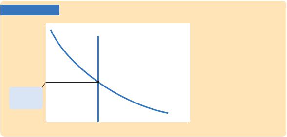
FIGURE 5-8
Real exchange |
S 2 I |
rate, e |
Equilibrium real exchange rate
NX(e)
How the Real Exchange Rate Is Determined The real exchange rate is determined by the intersection of the vertical line representing saving minus investment and the downward-sloping net-exports schedule. At this intersection, the quantity of dollars supplied for the flow of capital abroad equals the quantity of dollars demanded for the net export of goods and services.
Net exports, NX
foreigners who want dollars to buy our goods. At the equilibrium real exchange rate, the supply of dollars available from the net capital outflow balances the demand for dollars by foreigners buying our net exports.
How Policies Influence the Real Exchange Rate
We can use this model to show how the changes in economic policy we discussed earlier affect the real exchange rate.
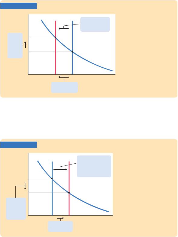
Fiscal Policy at Home What happens to the real exchange rate if the government reduces national saving by increasing government purchases or cutting taxes? As we discussed earlier, this reduction in saving lowers S – I and thus NX. That is, the reduction in saving causes a trade deficit.
Figure 5-9 shows how the equilibrium real exchange rate adjusts to ensure that NX falls. The change in policy shifts the vertical S − I line to the left, lowering the supply of dollars to be invested abroad. The lower supply causes the equilibrium real exchange rate to rise from e1 to e2—that is, the dollar becomes more valuable. Because of the rise in the value of the dollar, domestic goods become more expensive relative to foreign goods, which causes exports to fall and imports to rise. The change in exports and the change in imports both act to reduce net exports.
Fiscal Policy Abroad What happens to the real exchange rate if foreign governments increase government purchases or cut taxes? This change in fiscal policy reduces world saving and raises the world interest rate. The increase in the world interest rate reduces domestic investment I, which
140 | P A R T I I Classical Theory: The Economy in the Long Run
FIGURE 5-9
Real exchange |
S2 − I |
S1 − I |
|
rate, e |
1. A reduction in |
||
|
|
|
saving reduces the |
|
|
|
supply of dollars, ... |
2. ... e which 2 raises
the real exchange e1 rate ...
NX(e)
NX2 |
NX1 |
Net exports, NX |
3. ... and causes net exports to fall.
The Impact of Expansionary Fiscal Policy at Home on the Real Exchange Rate
Expansionary fiscal policy at home, such as an increase in government purchases or a cut in taxes, reduces national saving. The fall in saving
reduces the supply of dollars to be exchanged into foreign currency, from S1 − I to S2 − I. This shift raises the equilibrium real exchange rate from e1 to e2.
raises S − I and thus NX. That is, the increase in the world interest rate causes a trade surplus.
Figure 5-10 shows that this change in policy shifts the vertical S − I line to the right, raising the supply of dollars to be invested abroad. The equilibrium real
FIGURE 5-10
Real exchange rate, e
e1
e2
2. ... causes the real exchange rate to
fall, ...
S − I(r*1) |
S − I(r*2) |
1. An increase in world |
|
|
interest rates reduces |
|
|
investment, which |
|
|
increases the supply |
|
|
of dollars, ... |
NX(e)
NX1 |
NX2 |
Net exports, NX |
The Impact of Expansionary Fiscal Policy Abroad on the Real Exchange Rate
Expansionary fiscal policy abroad reduces world saving and raises
the world interest rate from r*1 to
r*. The increase in the world inter-
2
est rate reduces investment at home, which in turn raises the supply of dollars to be exchanged into foreign currencies. As a result, the equilibrium real exchange rate falls from e1 to e2.
3. ... and raises net exports.

C H A P T E R 5 The Open Economy | 141
exchange rate falls. That is, the dollar becomes less valuable, and domestic goods become less expensive relative to foreign goods.
Shifts in Investment Demand What happens to the real exchange rate if investment demand at home increases, perhaps because Congress passes an investment tax credit? At the given world interest rate, the increase in investment demand leads to higher investment. A higher value of I means lower values of S − I and NX. That is, the increase in investment demand causes a trade deficit.
Figure 5-11 shows that the increase in investment demand shifts the vertical S − I line to the left, reducing the supply of dollars to be invested abroad. The
FIGURE 5-11
Real exchange |
|
|
|
|
||
rate, e |
|
S − |
I2 |
S − |
I1 |
1. An increase in |
|
|
|||||
|
|
|
|
|
|
|
|
|
|
|
|
|
investment reduces |
|
|
|
|
|
|
the supply of dollars, ... |
2. ... |
e2 |
|
|
|
|
|
which |
|
|
|
|
|
|
raises the |
|
|
|
|
|
|
exchange |
e1 |
|
|
|
|
|
rate ... |
|
|
|
|
|
|
|
|
|
|
|
|
NX(e) |
|
|
|
|
|
|
|
|
|
NX2 |
NX1 |
Net exports, NX |
||
|
|
3. ... and reduces |
|
|||
|
|
net exports. |
|
|
|
|
The Impact of an Increase in Investment Demand on the Real Exchange Rate An increase in investment demand raises the quantity of domestic investment from I1 to I2. As a result, the supply of dollars to be exchanged into foreign currencies falls from S − I1 to S − I2. This fall in supply raises the equilibrium real exchange rate from e1 to e2.
equilibrium real exchange rate rises. Hence, when the investment tax credit makes investing in the United States more attractive, it also increases the value of the U.S. dollars necessary to make these investments. When the dollar appreciates, domestic goods become more expensive relative to foreign goods, and net exports fall.
The Effects of Trade Policies
Now that we have a model that explains the trade balance and the real exchange rate, we have the tools to examine the macroeconomic effects of trade policies. Trade policies, broadly defined, are policies designed to influence directly the
142 | P A R T I I Classical Theory: The Economy in the Long Run
amount of goods and services exported or imported. Most often, trade policies take the form of protecting domestic industries from foreign competition— either by placing a tax on foreign imports (a tariff) or restricting the amount of goods and services that can be imported (a quota).
As an example of a protectionist trade policy, consider what would happen if the government prohibited the import of foreign cars. For any given real exchange rate, imports would now be lower, implying that net exports (exports minus imports) would be higher. Thus, the net-exports schedule shifts outward, as in Figure 5-12. To see the effects of the policy, we compare the old equilibrium and the new equilibrium. In the new equilibrium, the real exchange rate is higher, and net exports are unchanged. Despite the shift in the net-exports schedule, the equilibrium level of net exports remains the same, because the protectionist policy does not alter either saving or investment.
This analysis shows that protectionist trade policies do not affect the trade balance. This surprising conclusion is often overlooked in the popular debate over trade policies. Because a trade deficit reflects an excess of imports over exports, one might guess that reducing imports—such as by prohibiting the import of foreign cars—would reduce a trade deficit. Yet our model shows that protectionist policies lead only to an appreciation of the real exchange rate. The increase in the price of domestic goods relative to foreign goods tends to lower net exports by stimulating imports and depressing exports. Thus, the
FIGURE 5-12
Real exchange
rate, e S − I
1. Protectionist policies raise the demand
for net exports ...
2. ... and e2 raise the exchange
rate ... e1
NX(e)2
NX(e)1
= Net exports, NX
NX1 NX2
The Impact of Protectionist Trade Policies on the Real Exchange Rate A protectionist trade policy, such as a ban on imported cars, shifts the netexports schedule from NX(e)1 to NX(e)2, which raises the real exchange rate from e1 to e2. Notice that, despite the shift in the net-exports schedule, the equilibrium level of net exports is unchanged.
3. ... but leave net exports unchanged.
C H A P T E R 5 The Open Economy | 143
appreciation offsets the increase in net exports that is directly attributable to the trade restriction.
Although protectionist trade policies do not alter the trade balance, they do affect the amount of trade. As we have seen, because the real exchange rate appreciates, the goods and services we produce become more expensive relative to foreign goods and services. We therefore export less in the new equilibrium. Because net exports are unchanged, we must import less as well. (The appreciation of the exchange rate does stimulate imports to some extent, but this only partly offsets the decrease in imports due to the trade restriction.) Thus, protectionist policies reduce both the quantity of imports and the quantity of exports.
This fall in the total amount of trade is the reason economists almost always oppose protectionist policies. International trade benefits all countries by allowing each country to specialize in what it produces best and by providing each country with a greater variety of goods and services. Protectionist policies diminish these gains from trade. Although these policies benefit certain groups within society—for example, a ban on imported cars helps domestic car producers—society on average is worse off when policies reduce the amount of international trade.
The Determinants of the Nominal Exchange Rate
Having seen what determines the real exchange rate, we now turn our attention to the nominal exchange rate—the rate at which the currencies of two countries trade. Recall the relationship between the real and the nominal exchange rate:
Real |
|
Nominal |
Ratio of |
Exchange = Exchange × Price |
|||
Rate |
|
Rate |
Levels |
e |
= |
e |
× (P/P *). |
We can write the nominal exchange rate as
e = e × (P */P ).
This equation shows that the nominal exchange rate depends on the real exchange rate and the price levels in the two countries. Given the value of the real exchange rate, if the domestic price level P rises, then the nominal exchange rate e will fall: because a dollar is worth less, a dollar will buy fewer yen. However, if the Japanese price level P * rises, then the nominal exchange rate will increase: because the yen is worth less, a dollar will buy more yen.
It is instructive to consider changes in exchange rates over time. The exchange rate equation can be written
% Change in e = % Change in e + % Change in P * − % Change in P.

144 | P A R T I I Classical Theory: The Economy in the Long Run
The percentage change in e is the change in the real exchange rate. The percentage change in P is the domestic inflation rate p, and the percentage change in P* is the foreign country’s inflation rate p*. Thus, the percentage change in the nominal exchange rate is
% Change in e = % Change in e |
+ (p* − p) |
|
Percentage Change in |
= Percentage Change in |
+ Difference in |
Nominal Exchange Rate |
Real Exchange Rate |
Inflation Rates. |
This equation states that the percentage change in the nominal exchange rate between the currencies of two countries equals the percentage change in the real exchange rate plus the difference in their inflation rates. If a country has a high rate of inflation relative to the United States, a dollar will buy an increasing amount of the foreign currency over time. If a country has a low rate of inflation relative to the United States, a dollar will buy a decreasing amount of the foreign currency over time.
This analysis shows how monetary policy affects the nominal exchange rate. We know from Chapter 4 that high growth in the money supply leads to high inflation. Here, we have just seen that one consequence of high inflation is a depreciating currency: high p implies falling e. In other words, just as growth in the amount of money raises the price of goods measured in terms of money, it also tends to raise the price of foreign currencies measured in terms of the domestic currency.
CASE STUDY
Inflation and Nominal Exchange Rates
If we look at data on exchange rates and price levels of different countries, we quickly see the importance of inflation for explaining changes in the nominal exchange rate. The most dramatic examples come from periods of very high inflation. For example, the price level in Mexico rose by 2,300 percent from 1983 to 1988. Because of this inflation, the number of pesos a person could buy with a U.S. dollar rose from 144 in 1983 to 2,281 in 1988.
The same relationship holds true for countries with more moderate inflation. Figure 5-13 is a scatterplot showing the relationship between inflation and the exchange rate for 15 countries. On the horizontal axis is the difference between each country’s average inflation rate and the average inflation rate of the United States (p* − p). On the vertical axis is the average percentage change in the exchange rate between each country’s currency and the U.S. dollar (percentage change in e). The positive relationship between these two variables is clear in this figure. Countries with relatively high inflation tend to have depreciating currencies (you can buy more of them with your dollars over time), and countries with relatively low inflation tend to have appreciating currencies (you can buy less of them with your dollars over time).
As an example, consider the exchange rate between Swiss francs and U.S. dollars. Both Switzerland and the United States have experienced inflation over the past thirty years, so both the franc and the dollar buy fewer goods than they once