414 | P A R T I V Business Cycle Theory: The Economy in the Short Run

The Nominal Interest Rate: The Monetary-Policy Rule

The last piece of the model is the equation for monetary policy. We assume that the central bank sets a target for the nominal interest rate it based on inflation and output using this rule:

poses, target inflation can be assumed to be constant, but we will keep a time subscript on this variable so we can examine later what happens when the central bank changes its target.) Two key policy parameters are vp and vY, which are both assumed to be greater than zero. They indicate how much the central bank allows the interest rate target to respond to fluctuations in inflation and output. The larger the value of vp, the more responsive the central bank is to the deviation of inflation from its target; the larger the value of vY, the more responsive the central bank is to the deviation of income from its natural level. Recall that r, the constant in this equation, is the natural rate of interest (the real interest rate at which, in the absence of any shock, the demand for goods and services equals the natural level of output). This equation tells us how the central bank uses monetary policy to respond to any situation it faces. That is, it tells us how the target for the nominal interest rate chosen by the central bank responds to macroeconomic conditions.

To interpret this equation, it is best to focus not just on the nominal interest rate it but also on the real interest rate rt. Recall that the real interest rate, rather than the nominal interest rate, influences the demand for goods and services. So, although the central bank sets a target for the nominal interest rate it, the bank’s influence on the economy works through the real interest rate rt. By definition,

natural level (Yt = Yt), the last two terms in the equation are zero, and so the real

At this point, one might naturally ask: what about the money supply? In previous chapters, such as Chapters 10 and 11, the money supply was typically taken to be the policy instrument of the central bank, and the interest rate adjusted to bring money supply and money demand into equilibrium. Here, we turn that logic on its head. The central bank is assumed to set a target for the nominal interest rate. It then adjusts the money supply to whatever level is necessary to ensure that the equilibrium interest rate (which balances money supply and demand) hits the target.

The main advantage of using the interest rate, rather than the money supply, as the policy instrument in the dynamic AD –AS model is that it is more realistic. Today, most central banks, including the Federal Reserve, set a short-term target for the nominal interest rate. Keep in mind, though, that

C H A P T E R 1 4 A Dynamic Model of Aggregate Demand and Aggregate Supply | 415

hitting that target requires adjustments in the money supply. For this model, we do not need to specify the equilibrium condition for the money market, but we should remember that it is lurking in the background. When a central bank decides to change the interest rate, it is also committing itself to adjust the money supply accordingly.

CASE STUDY

The Taylor Rule

If you wanted to set interest rates to achieve low, stable inflation while avoiding large fluctuations in output and employment, how would you do it? This is exactly the question that the governors of the Federal Reserve must ask themselves every day. The short-term policy instrument that the Fed now sets is the federal funds rate—the short-term interest rate at which banks make loans to one another. Whenever the Federal Open Market Committee meets, it chooses a target for the federal funds rate. The Fed’s bond traders are then told to conduct open-market operations to hit the desired target.

The hard part of the Fed’s job is choosing the target for the federal funds rate. Two general guidelines are clear. First, when inflation heats up, the federal funds rate should rise. An increase in the interest rate will mean a smaller money supply and, eventually, lower investment, lower output, higher unemployment, and reduced inflation. Second, when real economic activity slows—as reflected in real GDP or unemployment—the federal funds rate should fall. A decrease in the interest rate will mean a larger money supply and, eventually, higher investment, higher output, and lower unemployment. These two guidelines are represented by the monetary-policy equation in the dynamic AD –AS model.

The Fed needs to go beyond these general guidelines, however, and decide exactly how much to respond to changes in inflation and real economic activity. Stanford University economist John Taylor has proposed the following rule for the federal funds rate:1

Nominal Federal Funds Rate = Inflation + 2.0

+ 0.5 (Inflation − 2.0) + 0.5 (GDP gap).

The GDP gap is the percentage by which real GDP deviates from an estimate of its natural level. (For consistency with our dynamic AD –AS model, the GDP gap here is taken to be positive if GDP rises above its natural level and negative if it falls below it.)

According to the Taylor rule, the real federal funds rate—the nominal rate minus inflation—responds to inflation and the GDP gap. According to this rule,

1 John B. Taylor,“Discretion Versus Policy Rules in Practice,” Carnegie-Rochester Conference Series on Public Policy 39 (1993): 195–214.

416 | P A R T I V Business Cycle Theory: The Economy in the Short Run

the real federal funds rate equals 2 percent when inflation is 2 percent and GDP is at its natural level. The first constant of 2 percent in this equation can be interpreted as an estimate of the natural rate of interest r, and the second constant of 2 percent subtracted from inflation can be interpreted as the Fed’s inflation tar-

get p*. For each percentage point that inflation rises above 2 percent, the real

t

federal funds rate rises by 0.5 percent. For each percentage point that real GDP rises above its natural level, the real federal funds rate rises by 0.5 percent. If inflation falls below 2 percent or GDP moves below its natural level, the real federal funds rate falls accordingly.

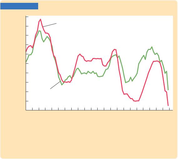
In addition to being simple and reasonable, the Taylor rule for monetary policy also resembles actual Fed behavior in recent years. Figure 14-1 shows the actual nominal federal funds rate and the target rate as determined by Taylor’s proposed rule. Notice how the two series tend to move together. John Taylor’s monetary rule may be more than an academic suggestion. To some degree, it may be the rule that the Federal Reserve governors have been subconsciously following. ■

FIGURE 14-1

Percent 10

Actual

9

8

7

6

5

4

3

2Taylor’s rule

1

The Federal Funds Rate: Actual and Suggested This figure shows the federal funds rate set by the Federal Reserve and the target rate that John Taylor’s rule for monetary policy would recommend. Notice that the two series move closely together.

Source: Federal Reserve Board, U.S. Department of Commerce, U.S. Department of Labor, and author’s calculations. To implement the Taylor rule, the inflation rate is measured as the percentage change in the GDP deflator over the previous four quarters, and the GDP gap is measured as negative two times the deviation of the unemployment rate from its natural rate (as shown in Figure 6-1).