C H A P T E R 1 4 A Dynamic Model of Aggregate Demand and Aggregate Supply | 423

aggregate supply curve in that period, which in turn affects output and inflation in period t + 1, which then affects expected inflation in period t + 2, and so on.

These linkages of economic outcomes across time periods will become clear as we work through a series of examples.

14-3 Using the Model

Let’s now use the dynamic AD –AS model to analyze how the economy

assume that the economy always begins in long-run equilibrium and is then subject to a change in one of the exogenous variables. We also assume that the other exogenous variables are held constant.

Long-Run Growth

−

The economy’s natural level of output Yt changes over time because of pop-

ulation growth, capital accumulation, and technological progress, as discussed

−

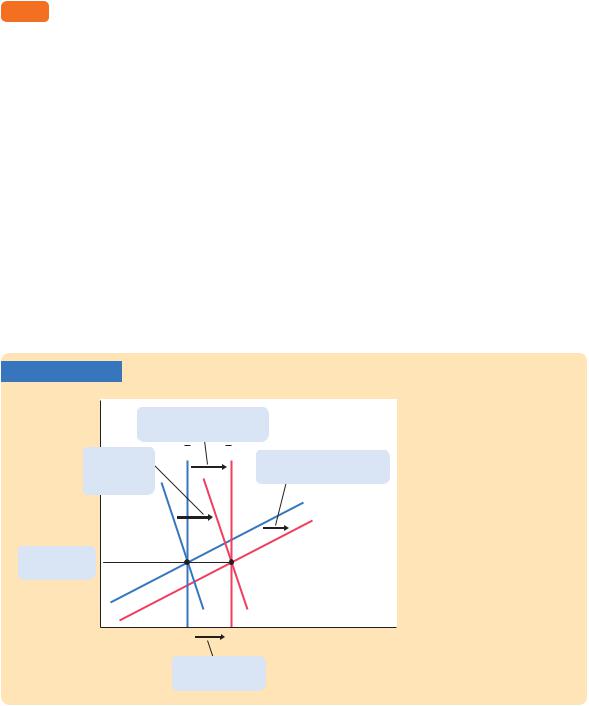
in Chapters 7 and 8. Figure 14-5 illustrates the effect of an increase in Yt. Because this variable affects both the dynamic aggregate demand curve and

the dynamic aggregate supply curve, both curves shift. In fact, they both shift

−

to the right by exactly the amount that Yt has increased.

424 | P A R T I V Business Cycle Theory: The Economy in the Short Run

The shifts in these curves move the economy’s equilibrium in the figure from

The story behind these conclusions is as follows: When the natural level of output increases, the economy can produce a larger quantity of goods and services. This is represented by the rightward shift in the dynamic aggregate supply curve. At the same time, the increase in the natural level of output makes people richer. Other things equal, they want to buy more goods and services. This is represented by the rightward shift in the dynamic aggregate demand curve. The simultaneous shifts in supply and demand increase the economy’s output without putting either upward or downward pressure on inflation. In this way, the economy can experience long-run growth and a stable inflation rate.

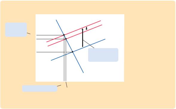
A Shock to Aggregate Supply

Consider now a shock to aggregate supply. In particular, suppose that ut rises to 1 percent for one period and subsequently returns to zero. This shock to the Phillips curve might occur, for example, because an international oil cartel pushes up prices or because new union agreements raise wages and, thereby, the costs of production.

expected inflation Et −1pt and current economic activity, as measured by Yt − Yt. Figure 14-6 shows the result. In period t, when the shock occurs, the dynam-

ic aggregate supply curve shifts upward from DASt −1 to DASt. To be precise, the

C H A P T E R 1 4 A Dynamic Model of Aggregate Demand and Aggregate Supply | 425

curve shifts upward by exactly the size of the shock, which we assumed to be 1 percentage point. Because the supply shock ut is not a variable in the dynamic aggregate demand equation, the DAD curve is unchanged. Therefore, the economy moves along the dynamic aggregate demand curve from point A to point B. As the figure illustrates, the supply shock in period t causes inflation to rise to pt and output to fall to Yt.

These effects work in part through the reaction of monetary policy to the shock. When the supply shock causes inflation to rise, the central bank responds by following its policy rule and raising nominal and real interest rates. The higher real interest rate reduces the quantity of goods and services demanded, which depresses output below its natural level. (This series of events is represented by the movement along the DAD curve from point A to point B.) The lower level of output dampens the inflationary pressure to some degree, so inflation rises somewhat less than the initial shock.

426 | P A R T I V Business Cycle Theory: The Economy in the Short Run

In the periods after the shock occurs, expected inflation is higher because expectations depend on past inflation. In period t + 1, for instance, the economy is at point C. Even though the shock variable ut returns to its normal value of zero, the dynamic aggregate supply curve does not immediately return to its initial position. Instead, it slowly shifts back downward toward its initial position DASt −1 as a lower level of economic activity reduces inflation and thereby expectations of future inflation. Throughout this process, output remains below its natural level.

Figure 14-7 shows the time paths of the key variables in the model in response to the shock. (These simulations are based on realistic parameter values: see the