C H A P T E R 1 0 Aggregate Demand I: Building the IS–LM Model | 289
The two parts of the IS –LM model are, not surprisingly, the IS curve and the LM curve. IS stands for “investment’’ and “saving,’’ and the IS curve represents what’s going on in the market for goods and services (which we first discussed in Chapter 3). LM stands for “liquidity’’ and “money,’’ and the LM curve represents what’s happening to the supply and demand for money (which we first discussed in Chapter 4). Because the interest rate influences both investment and money demand, it is the variable that links the two halves of the IS –LM model. The model shows how interactions between the goods and money markets determine the position and slope of the aggregate demand curve and, therefore, the level of national income in the short run.1
10-1 The Goods Market and the IS Curve
The IS curve plots the relationship between the interest rate and the level of income that arises in the market for goods and services. To develop this relationship, we start with a basic model called the Keynesian cross. This model is the simplest interpretation of Keynes’s theory of how national income is determined and is a building block for the more complex and realistic IS–LM model.
The Keynesian Cross
In The General Theory Keynes proposed that an economy’s total income was, in the short run, determined largely by the spending plans of households, businesses, and government. The more people want to spend, the more goods and services firms can sell. The more firms can sell, the more output they will choose to produce and the more workers they will choose to hire. Keynes believed that the problem during recessions and depressions was inadequate spending. The Keynesian cross is an attempt to model this insight.
Planned Expenditure We begin our derivation of the Keynesian cross by drawing a distinction between actual and planned expenditure. Actual expenditure is the amount households, firms, and the government spend on goods and services, and as we first saw in Chapter 2, it equals the economy’s gross domestic product (GDP). Planned expenditure is the amount households, firms, and the government would like to spend on goods and services.
Why would actual expenditure ever differ from planned expenditure? The answer is that firms might engage in unplanned inventory investment because their sales do not meet their expectations. When firms sell less of their product than they planned, their stock of inventories automatically rises; conversely, when
1 The IS-LM model was introduced in a classic article by the Nobel Prize–winning economist John R. Hicks, “Mr. Keynes and the Classics: A Suggested Interpretation,’’ Econometrica 5 (1937): 147–159.

290 | P A R T I V Business Cycle Theory: The Economy in the Short Run
firms sell more than planned, their stock of inventories falls. Because these unplanned changes in inventory are counted as investment spending by firms, actual expenditure can be either above or below planned expenditure.
Now consider the determinants of planned expenditure. Assuming that the economy is closed, so that net exports are zero, we write planned expenditure PE as the sum of consumption C, planned investment I, and government purchases G:
PE = C + I + G.
To this equation, we add the consumption function
C = C(Y − T ).
This equation states that consumption depends on disposable income (Y − T ), which is total income Y minus taxes T. To keep things simple, for now we take planned investment as exogenously fixed:
I = I−.
Finally, as in Chapter 3, we assume that fiscal policy—the levels of government purchases and taxes—is fixed:
= −
G G ,
= −
T T .
Combining these five equations, we obtain
= − − − −
PE C(Y T ) + I + G .
This equation shows that planned expenditure is a function of income Y, the |
− |
− |
− |
level of planned investment I , and the fiscal policy variables G and T .
Figure 10-2 graphs planned expenditure as a function of the level of income. This line slopes upward because higher income leads to higher consumption and
FIGURE 10-2
Planned |
|
expenditure, PE |
Planned expenditure, PE C(Y T) I G |
MPC
$1
Planned Expenditure as a Function of Income Planned expenditure PE depends on income because higher income leads to higher consumption, which is part of planned expenditure. The slope of the planned-expenditure function is the marginal propensity to consume, MPC.
C H A P T E R 1 0 Aggregate Demand I: Building the IS–LM Model | 291
thus higher planned expenditure. The slope of this line is the marginal propensity to consume, MPC: it shows how much planned expenditure increases when income rises by $1. This planned-expenditure function is the first piece of the model called the Keynesian cross.
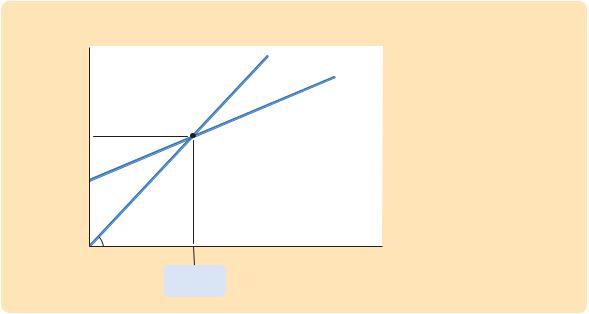
The Economy in Equilibrium The next piece of the Keynesian cross is the assumption that the economy is in equilibrium when actual expenditure equals planned expenditure. This assumption is based on the idea that when people’s plans have been realized, they have no reason to change what they are doing. Recalling that Y as GDP equals not only total income but also total actual expenditure on goods and services, we can write this equilibrium condition as
Actual Expenditure = Planned Expenditure
Y = PE.
The 45-degree line in Figure 10-3 plots the points where this condition holds. With the addition of the planned-expenditure function, this diagram becomes the Keynesian cross. The equilibrium of this economy is at point A, where the planned-expenditure function crosses the 45-degree line.
How does the economy get to equilibrium? In this model, inventories play an important role in the adjustment process. Whenever an economy is not in equilibrium, firms experience unplanned changes in inventories, and this induces them to change production levels. Changes in production in turn influence total income and expenditure, moving the economy toward equilibrium.
For example, suppose the economy finds itself with GDP at a level greater than the equilibrium level, such as the level Y1 in Figure 10-4. In this case, planned expenditure PE1 is less than production Y1, so firms are selling less than
|
FIGURE 10-3 |
|
|
Expenditure |
Actual expenditure, |
|
(Planned, PE |
|
Y PE |
|
Actual, Y) |
|
|
|
|
G |
The Keynesian Cross The equilibrium in the Keynesian cross is the point at which income (actual expenditure) equals planned expenditure (point A).
292 | P A R T I V Business Cycle Theory: The Economy in the Short Run
FIGURE 10-4 |
|
|
Expenditure |
|
|
Actual expenditure |
(Planned, PE, |
|
|
|
|
|
Actual, Y) |
|
|
|
Y1 |
Unplanned |
|
|
drop in |
|
|
|
|
|
PE1 |
inventory |
|
Planned expenditure |
causes |
|
|
income to rise. |
|
|
PE2 |
|
|
Unplanned |
|
|
|
Y2 |
|
|
inventory |
|
|
accumulation |
|
|
|
|
|
|
causes |
|
45º |
|
income to fall. |
|
|
|
|
Y2 |
Y1 |
Income, output, Y |
|
|
Equilibrium |
|
|
|
income |
|
The Adjustment to Equilibrium in the Keynesian Cross If firms are producing at level Y1, then planned expenditure PE1 falls short of production, and firms accumulate inventories. This inventory accumulation induces firms to decrease production. Similarly, if
firms are producing at level Y2, then planned expenditure PE2 exceeds production, and firms run down their inventories. This fall in inventories induces firms to increase production. In both cases, the firms’ decisions drive the economy toward equilibrium.
they are producing. Firms add the unsold goods to their stock of inventories. This unplanned rise in inventories induces firms to lay off workers and reduce production; these actions in turn reduce GDP. This process of unintended inventory accumulation and falling income continues until income Y falls to the equilibrium level.
Similarly, suppose GDP is at a level lower than the equilibrium level, such as the level Y2 in Figure 10-4. In this case, planned expenditure PE2 is greater than production Y2. Firms meet the high level of sales by drawing down their inventories. But when firms see their stock of inventories dwindle, they hire more workers and increase production. GDP rises, and the economy approaches the equilibrium.
In summary, the Keynesian cross shows how income Y is determined for given levels of planned investment I and fiscal policy G and T. We can use this model to show how income changes when one of these exogenous variables changes.
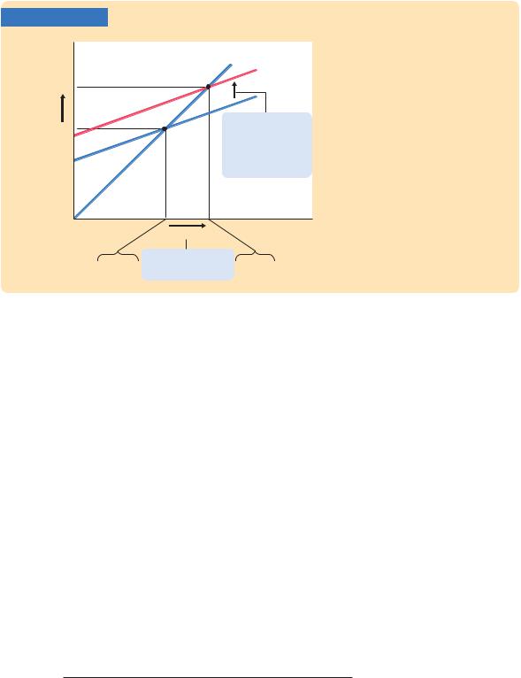
Fiscal Policy and the Multiplier: Government Purchases Consider how changes in government purchases affect the economy. Because government purchases are one component of expenditure, higher government purchases result in higher planned expenditure for any given level of income. If government purchases rise by G, then the planned-expenditure schedule shifts upward by G, as in Figure 10-5. The equilibrium of the economy moves from point A to point B.
This graph shows that an increase in government purchases leads to an even greater increase in income. That is, Y is larger than G. The ratio Y/ G is called the government-purchases multiplier; it tells us how much income rises in response to a $1 increase in government purchases. An implication of the Keynesian cross is that the government-purchases multiplier is larger than 1.
C H A P T E R 1 0 Aggregate Demand I: Building the IS–LM Model | 293
FIGURE 10-5
Expenditure
|
Actual expenditure |
|
B |
Planned |
|
expenditure |
PE2 Y2 |
|
G |
Y |
|
|
PE1 Y1 |
|
1. An increase |
A |
in government |
purchases shifts planned expenditure upward, ...
 45º
45º
Income, output, Y
Y
|
PE1 Y1 |
2. ...which increases |
PE2 |
Y2 |
|
equilibrium income. |
|
|
|
|
An Increase in Government Purchases in the Keynesian Cross
An increase in government purchases of G raises planned expenditure by that amount for any given level of income. The equilibrium moves from point A to point B, and income rises from Y1 to Y2. Note that the increase in income Y exceeds the increase in government purchases G. Thus, fiscal policy has a multiplied effect on income.
Why does fiscal policy have a multiplied effect on income? The reason is that, according to the consumption function C = C(Y − T ), higher income causes higher consumption. When an increase in government purchases raises income, it also raises consumption, which further raises income, which further raises consumption, and so on. Therefore, in this model, an increase in government purchases causes a greater increase in income.
How big is the multiplier? To answer this question, we trace through each step of the change in income. The process begins when expenditure rises by G, which implies that income rises by G as well. This increase in income in turn raises consumption by MPC × G, where MPC is the marginal propensity to consume. This increase in consumption raises expenditure and income once again. This second increase in income of MPC × G again raises consumption, this time by MPC × (MPC × G ), which again raises expenditure and income, and so on. This feedback from consumption to income to consumption continues indefinitely. The total effect on income is
Initial Change in Government Purchases = |
|
DG |
First Change in Consumption |
= MPC × DG |
Second Change in Consumption |
= MPC2 |
× |
D |
G |
. |
= MPC3 |
. |
D |
Third Change in Consumption |
× |
G |
. |
|
. |
|
. |
|
. |
|
DY = (1 + MPC + MPC2 + MPC3 + . . .)DG.
294 | P A R T I V Business Cycle Theory: The Economy in the Short Run
The government-purchases multiplier is
DY/DG = 1 + MPC + MPC2 + MPC3 + . . .
This expression for the multiplier is an example of an infinite geometric series. A result from algebra allows us to write the multiplier as2
DY/DG = 1/(1 − MPC ).
For example, if the marginal propensity to consume is 0.6, the multiplier is
DY/DG = 1 + 0.6 + 0.62 + 0.63 + . . .
= 1/(1 − 0.6)
= 2.5.
In this case, a $1.00 increase in government purchases raises equilibrium income by $2.50.3
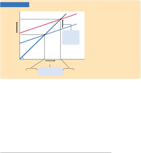
Fiscal Policy and the Multiplier: Taxes Consider now how changes in taxes affect equilibrium income. A decrease in taxes of T immediately raises disposable income Y − T by T and, therefore, increases consumption by MPC × T. For any given level of income Y, planned expenditure is now higher. As Figure 10-6 shows, the planned-expenditure schedule shifts upward by MPC × T.
The equilibrium of the economy moves from point A to point B.
2 Mathematical note: We prove this algebraic result as follows. For x < 1, let z = 1 + x + x2 + . . . .
Multiply both sides of this equation by x:
xz = x + x2 + x3 + . . . .
Subtract the second equation from the first:
z − xz = 1.
Rearrange this last equation to obtain
z(1 − x) = 1,
which implies
z = 1/(1 − x).
This completes the proof.
3 Mathematical note: The government-purchases multiplier is most easily derived using a little calculus. Begin with the equation
Y = C(Y − T ) + I + G.
Holding T and I fixed, differentiate to obtain
dY = C′dY + dG,
and then rearrange to find
dY/dG = 1/(1 − C ′). This is the same as the equation in the text.
|
C H A P T E R |
1 0 Aggregate Demand I: Building the IS–LM Model | 295 |
FIGURE 10-6 |
|
|
|
|
|
Expenditure |
Actual expenditure |
|
A Decrease in Taxes in the |
|
Planned |
Keynesian Cross A decrease in |
PE2 Y2 |
B |
|
|
|
expenditure |
taxes of T raises planned expendi- |
|
|
MPC |
T |
ture by MPC × |
T for any given |
Y |
|
|
|
level of income. The equilibrium |
|
|
|
moves from point A to point B, and |
|
|
|
|
PE1 Y1 |
|
1. A tax cut |
income rises from Y1 to Y2. Again, |
A |
shifts planned |
fiscal policy has a multiplied effect |
|
expenditure |
on income. |
|
|
|
|
|
|
upward, ... |
|
|
45º |
|
|
|
|
|
|
Y |
|
Income, |
|
|
|
|
output, Y |
|
|
|
|
|
|
|
2. ...which increases |
PE2 Y2 |
PE1 Y1 equilibrium income. |
Just as an increase in government purchases has a multiplied effect on income, so does a decrease in taxes. As before, the initial change in expenditure, now MPC × T, is multiplied by 1/(1 − MPC ). The overall effect on income of the change in taxes is
Y/ T = −MPC/(1 − MPC ).
This expression is the tax multiplier, the amount income changes in response to a $1 change in taxes. (The negative sign indicates that income moves in the opposite direction from taxes.) For example, if the marginal propensity to consume is 0.6, then the tax multiplier is
Y/ T = −0.6/(1 − 0.6) = −1.5.
In this example, a $1.00 cut in taxes raises equilibrium income by $1.50.4
4 Mathematical note: As before, the multiplier is most easily derived using a little calculus. Begin with the equation
Y = C(Y – T ) + I + G.
Holding I and G fixed, differentiate to obtain
dY = C ′(dY − dT ),
and then rearrange to find
dY/dT = –C ′/(1 − C ′). This is the same as the equation in the text.
296 | P A R T I V Business Cycle Theory: The Economy in the Short Run
CASE STUDY
Cutting Taxes to Stimulate the Economy:
The Kennedy and Bush Tax Cuts
When John F. Kennedy became president of the United States in 1961, he brought to Washington some of the brightest young economists of the day to work on his Council of Economic Advisers. These economists, who had been schooled in the economics of Keynes, brought Keynesian ideas to discussions of economic policy at the highest level.
One of the council’s first proposals was to expand national income by reducing taxes. This eventually led to a substantial cut in personal and corporate income taxes in 1964. The tax cut was intended to stimulate expenditure on consumption and investment and lead to higher levels of income and employment. When a reporter asked Kennedy why he advocated a tax cut, Kennedy replied,“To stimulate the economy. Don’t you remember your Economics 101?”
As Kennedy’s economic advisers predicted, the passage of the tax cut was followed by an economic boom. Growth in real GDP was 5.3 percent in 1964 and 6.0 percent in 1965. The unemployment rate fell from 5.7 percent in 1963 to 5.2 percent in 1964 and then to 4.5 percent in 1965.
Economists continue to debate the source of this rapid growth in the early 1960s. A group called supply-siders argues that the economic boom resulted from the incentive effects of the cut in income tax rates. According to supply-siders, when workers are allowed to keep a higher fraction of their earnings, they supply substantially more labor and expand the aggregate supply of goods and services. Keynesians, however, emphasize the impact of tax cuts on aggregate demand. Most likely, both views have some truth: Tax cuts stimulate aggregate supply by improving workers’ incentives and expand aggregate demand by raising households’ disposable income.
When George W. Bush was elected president in 2000, a major element of his platform was a cut in income taxes. Bush and his advisors used both supply-side and Keynesian rhetoric to make the case for their policy. (Full disclosure: The author of this textbook was one of Bush’s economic advisers from 2003 to 2005.) During the campaign, when the economy was doing fine, they argued that lower marginal tax rates would improve work incentives. But when the economy started to slow, and unemployment started to rise, the argument shifted to emphasize that the tax cut would stimulate spending and help the economy recover from the recession.
Congress passed major tax cuts in 2001 and 2003. After the second tax cut, the weak recovery from the 2001 recession turned into a robust one. Growth in real GDP was 4.4 percent in 2004. The unemployment rate fell from its peak of 6.3 percent in June 2003 to 5.4 percent in December 2004.
When President Bush signed the 2003 tax bill, he explained the measure using the logic of aggregate demand:“When people have more money, they can spend it on goods and services. And in our society, when they demand an additional good or a service, somebody will produce the good or a service. And when somebody produces that good or a service, it means somebody is more likely to be able to find a job.” The explanation could have come from an exam in Economics 101. ■
“Your Majesty, my voyage will not only forge a new route to the spices of the East but also create over three thousand new jobs.”
C H A P T E R 1 0 Aggregate Demand I: Building the IS–LM Model | 297
CASE STUDY
Increasing Government Purchases to Stimulate the Economy: The Obama Spending Plan
When President Barack Obama took office in January 2009, the economy was suffering from a significant recession. (The causes of this recession are discussed in a Case Study in the next chapter.) Even before he was inaugurated, the president and his advisers proposed a sizable stimulus package to increase aggregate demand. As proposed, the package would cost the federal government about $800 billion, or about 5 percent of annual GDP. The package included some tax cuts and higher transfer payments, but much of it was made up of increases in government purchases of goods and services.
Professional economists debated the merits of the plan. Advocates of the Obama plan argued that increased spending was better than reduced taxes because, accord-
ing to standard Keynesian theory, |
|
the government-purchases mul- |
|
tiplier exceeds the tax multipli- |
|
er. The reason for this difference |
Collection.YorkerNewThe© 1992 Dana Fradon cartoonbank.com.fromAll Rights Reserved. |
is simple: when the government |
ernment purchases multiplier is |
spends a dollar, that dollar gets |
|
spent, whereas when the gov- |
|
ernment gives households a tax |
|
cut of a dollar, some of that dol- |
|
lar might be saved. According |
|
to an analysis by Obama admin- |
|
istration economists, the gov- |
|
1.57, whereas the tax multiplier is only 0.99. Thus, they argued that increased government spend-
ing on roads, schools, and other infrastructure was the better route to increase aggregate demand and create jobs.
Other economists were more skeptical about the plan. One concern was that spending on infrastructure would take time, whereas tax cuts could occur more immediately. Infrastructure spending requires taking bids and signing contracts, and, even after the projects begin, they can take years to complete. The Congressional Budget Office estimated that only about 10 percent of the outlays would occur in the first nine months of 2009 and that a large fraction of outlays would be years away. By the time much of the stimulus went into effect, the recession might be well over.
In addition, some economists thought that using infrastructure spending to promote employment might conflict with the goal of obtaining the infrastructure that was most needed. Here is how Gary Becker, the Nobel Prize–winning economist, explained the concern on his blog:
Putting new infrastructure spending in depressed areas like Detroit might have a big stimulating effect since infrastructure building projects in these areas can utilize some of the considerable unemployed resources there. However, many of these