

C H A P T E R 3 National Income: Where It Comes From and Where It Goes | 61
In Chapter 2 we identified the four components of GDP:
■Consumption (C )
■Investment (I )
■Government purchases (G)
■Net exports (NX ).
The circular flow diagram contains only the first three components. For now, to simplify the analysis, we assume our economy is a closed economy—a country that does not trade with other countries. Thus, net exports are always zero. (We examine the macroeconomics of open economies in Chapter 5.)
A closed economy has three uses for the goods and services it produces. These three components of GDP are expressed in the national income accounts identity:
Y = C + I + G.
Households consume some of the economy’s output; firms and households use some of the output for investment; and the government buys some of the output for public purposes. We want to see how GDP is allocated among these three uses.
Consumption
When we eat food, wear clothing, or go to a movie, we are consuming some of the output of the economy. All forms of consumption together make up about two-thirds of GDP. Because consumption is so large, macroeconomists have devoted much energy to studying how households decide how much to consume. Chapter 17 examines this work in detail. Here we consider the simplest story of consumer behavior.
Households receive income from their labor and their ownership of capital, pay taxes to the government, and then decide how much of their after-tax income to consume and how much to save. As we discussed in Section 3-2, the income that households receive equals the output of the economy Y. The government then taxes households an amount T. (Although the government imposes many kinds of taxes, such as personal and corporate income taxes and sales taxes, for our purposes we can lump all these taxes together.) We define income after the payment of all taxes, Y − T, to be disposable income. Households divide their disposable income between consumption and saving.
We assume that the level of consumption depends directly on the level of disposable income. A higher level of disposable income leads to greater consumption. Thus,
C = C(Y − T ).
This equation states that consumption is a function of disposable income. The relationship between consumption and disposable income is called the consumption function.
62 | P A R T I I Classical Theory: The Economy in the Long Run
The marginal propensity to consume (MPC) is the amount by which consumption changes when disposable income increases by one dollar. The MPC is between zero and one: an extra dollar of income increases consumption, but by less than one dollar. Thus, if households obtain an extra dollar of income, they save a portion of it. For example, if the MPC is 0.7, then households spend 70 cents of each additional dollar of disposable income on consumer goods and services and save 30 cents.
Figure 3-6 illustrates the consumption function. The slope of the consumption function tells us how much consumption increases when disposable income increases by one dollar. That is, the slope of the consumption function is the MPC.
Investment
Both firms and households purchase investment goods. Firms buy investment goods to add to their stock of capital and to replace existing capital as it wears out. Households buy new houses, which are also part of investment. Total investment in the United States averages about 15 percent of GDP.
The quantity of investment goods demanded depends on the interest rate, which measures the cost of the funds used to finance investment. For an investment project to be profitable, its return (the revenue from increased future production of goods and services) must exceed its cost (the payments for borrowed funds). If the interest rate rises, fewer investment projects are profitable, and the quantity of investment goods demanded falls.
For example, suppose a firm is considering whether it should build a $1 million factory that would yield a return of $100,000 per year, or 10 percent. The firm compares this return to the cost of borrowing the $1 million. If the interest rate is below 10 percent, the firm borrows the money in financial markets
FIGURE 3-6
Consumption, C
Consumption
function
MPC
1
The Consumption Function The consumption function relates consumption C to disposable income Y − T. The marginal propensity to consume MPC is the amount by which consumption increases when disposable income increases by one dollar.
Disposable income, Y T
C H A P T E R 3 National Income: Where It Comes From and Where It Goes | 63
and makes the investment. If the interest rate is above 10 percent, the firm forgoes the investment opportunity and does not build the factory.
The firm makes the same investment decision even if it does not have to borrow the $1 million but rather uses its own funds. The firm can always deposit this money in a bank or a money market fund and earn interest on it. Building the factory is more profitable than depositing the money if and only if the interest rate is less than the 10 percent return on the factory.
A person wanting to buy a new house faces a similar decision. The higher the interest rate, the greater the cost of carrying a mortgage. A $100,000 mortgage costs $8,000 per year if the interest rate is 8 percent and $10,000 per year if the interest rate is 10 percent. As the interest rate rises, the cost of owning a home rises, and the demand for new homes falls.
When studying the role of interest rates in the economy, economists distinguish between the nominal interest rate and the real interest rate. This distinction is relevant when the overall level of prices is changing. The nominal interest rate is the interest rate as usually reported: it is the rate of interest that investors pay to borrow money. The real interest rate is the nominal interest rate corrected for the effects of inflation. If the nominal interest rate is 8 percent and the inflation rate is 3 percent, then the real interest rate is 5 percent. In Chapter 4 we discuss the relation between nominal and real interest rates in detail. Here it is sufficient to note that the real interest rate measures the true cost of borrowing and, thus, determines the quantity of investment.
We can summarize this discussion with an equation relating investment I to the real interest rate r:
I = I(r).
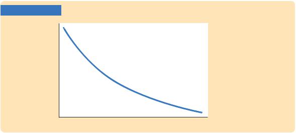
Figure 3-7 shows this investment function. It slopes downward, because as the interest rate rises, the quantity of investment demanded falls.
FIGURE 3-7
Real interest rate, r
Investment function, I(r)
The Investment Function The investment function relates the quantity of investment I to the real interest rate r. Investment depends on the real interest rate because the interest rate is the cost of borrowing. The investment function slopes downward: when the interest rate rises, fewer investment projects are profitable.
Quantity of investment, I

64 | P A R T I I Classical Theory: The Economy in the Long Run
FYI
The Many Different Interest Rates
If you look in the business section of a newspaper, you will find many different interest rates reported. By contrast, throughout this book, we will talk about “the” interest rate, as if there were only one interest rate in the economy. The only distinction we will make is between the nominal interest rate (which is not corrected for inflation) and the real interest rate (which is corrected for inflation). Almost all of the interest rates reported in the newspaper are nominal.
Why does the newspaper report so many interest rates? The various interest rates differ in three ways:
Term. Some loans in the economy are for short periods of time, even as short as overnight. Other loans are for thirty years or even longer. The interest rate on a loan depends on its term. Long-term interest rates are usually, but not always, higher than short-term interest rates.
Credit risk. In deciding whether to make a loan, a lender must take into account the probability that the borrower will
repay. The law allows borrowers to default on their loans by declaring bankruptcy. The higher the perceived probability of
default, the higher the interest rate. Because the safest credit risk is the government, government bonds tend to pay a low interest rate. At the other extreme, financially shaky corporations can raise funds only by issuing junk bonds, which pay a high interest rate to compensate for the high risk of default.
Tax treatment. The interest on different types of bonds is taxed differently. Most important, when state and local
governments issue bonds, called municipal bonds, the holders of the bonds do
not pay federal income tax on the interest income. Because of this tax advantage, municipal bonds pay a lower interest rate.
When you see two different interest rates in the newspaper, you can almost always explain the difference by considering the term, the credit risk, and the tax treatment of the loan.
Although there are many different interest rates in the economy, macroeconomists can usually ignore these distinctions. The various interest rates tend to move up and down together. For many purposes, we will not go far wrong by assuming there is only one interest rate.
Government Purchases
Government purchases are the third component of the demand for goods and services. The federal government buys guns, missiles, and the services of government employees. Local governments buy library books, build schools, and hire teachers. Governments at all levels build roads and other public works. All these transactions make up government purchases of goods and services, which account for about 20 percent of GDP in the United States.
These purchases are only one type of government spending. The other type is transfer payments to households, such as welfare for the poor and Social Security payments for the elderly. Unlike government purchases, transfer payments are not made in exchange for some of the economy’s output of goods and services. Therefore, they are not included in the variable G.

C H A P T E R 3 National Income: Where It Comes From and Where It Goes | 65
Transfer payments do affect the demand for goods and services indirectly. Transfer payments are the opposite of taxes: they increase households’ disposable income, just as taxes reduce disposable income. Thus, an increase in transfer payments financed by an increase in taxes leaves disposable income unchanged. We can now revise our definition of T to equal taxes minus transfer payments. Disposable income, Y − T, includes both the negative impact of taxes and the positive impact of transfer payments.
If government purchases equal taxes minus transfers, then G = T and the government has a balanced budget. If G exceeds T, the government runs a budget deficit, which it funds by issuing government debt—that is, by borrowing in the financial markets. If G is less than T, the government runs a budget surplus, which it can use to repay some of its outstanding debt.
Here we do not try to explain the political process that leads to a particular fiscal policy—that is, to the level of government purchases and taxes. Instead, we take government purchases and taxes as exogenous variables. To denote that these variables are fixed outside of our model of national income, we write
_
G = G.
_
T = T.
We do, however, want to examine the impact of fiscal policy on the endogenous variables, which are determined within the model. The endogenous variables here are consumption, investment, and the interest rate.
To see how the exogenous variables affect the endogenous variables, we must complete the model. This is the subject of the next section.
3-4 What Brings the Supply and
Demand for Goods and Services
Into Equilibrium?
We have now come full circle in the circular flow diagram, Figure 3-1. We began by examining the supply of goods and services, and we have just discussed the demand for them. How can we be certain that all these flows balance? In other words, what ensures that the sum of consumption, investment, and government purchases equals the amount of output produced? We will see that in this classical model, the interest rate is the price that has the crucial role of equilibrating supply and demand.
There are two ways to think about the role of the interest rate in the economy. We can consider how the interest rate affects the supply and demand for goods or services. Or we can consider how the interest rate affects the supply and demand for loanable funds. As we will see, these two approaches are two sides of the same coin.
66 | P A R T I I Classical Theory: The Economy in the Long Run
Equilibrium in the Market for Goods and Services:
The Supply and Demand for the Economy’s Output
The following equations summarize the discussion of the demand for goods and services in Section 3-3:
Y = C + I + G.
C = C(Y − T ).
I = I(r).
= –
G G.
= –
T T .
The demand for the economy’s output comes from consumption, investment, and government purchases. Consumption depends on disposable income; investment depends on the real interest rate; and government purchases and taxes are the exogenous variables set by fiscal policymakers.
To this analysis, let’s add what we learned about the supply of goods and services in Section 3-1. There we saw that the factors of production and the production function determine the quantity of output supplied to the economy:
= – –
Y F(K, L)
= –
Y.
Now let’s combine these equations describing the supply and demand for output. If we substitute the consumption function and the investment function into the national income accounts identity, we obtain
Y = C(Y − T ) + I(r) + G.
Because the variables G and T are fixed by policy, and the level of output Y is fixed by the factors of production and the production function, we can write
– |
– |
– |
– |
Y |
= C(Y |
− T ) + I(r) + G. |
|
This equation states that the supply of output equals its demand, which is the sum of consumption, investment, and government purchases.
Notice that the interest rate r is the only variable not already determined in the last equation. This is because the interest rate still has a key role to play: it must adjust to ensure that the demand for goods equals the supply. The greater the interest rate, the lower the level of investment, and thus the lower the demand for goods and services, C + I + G. If the interest rate is too high, then investment is too low and the demand for output falls short of the supply. If the interest rate is too low, then investment is too high and the demand exceeds the supply. At the equilibrium interest rate, the demand for goods and services equals the supply.
This conclusion may seem somewhat mysterious: how does the interest rate get to the level that balances the supply and demand for goods and services? The best way to answer this question is to consider how financial markets fit into the story.
C H A P T E R 3 National Income: Where It Comes From and Where It Goes | 67
Equilibrium in the Financial Markets:
The Supply and Demand for Loanable Funds
Because the interest rate is the cost of borrowing and the return to lending in financial markets, we can better understand the role of the interest rate in the economy by thinking about the financial markets. To do this, rewrite the national income accounts identity as
Y − C − G = I.
The term Y − C − G is the output that remains after the demands of consumers and the government have been satisfied; it is called national saving or simply saving (S ). In this form, the national income accounts identity shows that saving equals investment.
To understand this identity more fully, we can split national saving into two parts—one part representing the saving of the private sector and the other representing the saving of the government:
S = (Y − T − C ) + (T − G) = I.
The term (Y − T − C ) is disposable income minus consumption, which is private saving. The term (T − G) is government revenue minus government spending, which is public saving. (If government spending exceeds government revenue, then the government runs a budget deficit and public saving is negative.) National saving is the sum of private and public saving. The circular flow diagram in Figure 3-1 reveals an interpretation of this equation: this equation states that the flows into the financial markets (private and public saving) must balance the flows out of the financial markets (investment).
To see how the interest rate brings financial markets into equilibrium, substitute the consumption function and the investment function into the national income accounts identity:
Y − C(Y − T ) − G = I(r).
Next, note that G and T are fixed by policy and Y is fixed by the factors of production and the production function:
– |
– |
– – |
= I(r) |
Y |
− C(Y |
− T ) − G |
|
|
|
– |
= I(r). |
|
|
S |
The left-hand side of this equation shows that national saving depends on income Y and the fiscal-policy variables G and T. For fixed values of Y, G, and T, national saving S is also fixed. The right-hand side of the equation shows that investment depends on the interest rate.
Figure 3-8 graphs saving and investment as a function of the interest rate. The saving function is a vertical line because in this model saving does not depend on the interest rate (we relax this assumption later). The investment function slopes downward: as the interest rate decreases, more investment projects become profitable.
From a quick glance at Figure 3-8, one might think it was a supply-and-demand diagram for a particular good. In fact, saving and investment can be interpreted in terms of supply and demand. In this case, the “good” is loanable funds, and its