324 | P A R T I V Business Cycle Theory: The Economy in the Short Run

The IS–LM Model in the Short Run and Long Run

The IS –LM model is designed to explain the economy in the short run when the price level is fixed. Yet, now that we have seen how a change in the price level influences the equilibrium in the IS –LM model, we can also use the model to describe the economy in the long run when the price level adjusts to ensure that the economy produces at its natural rate. By using the IS –LM model to describe the long run, we can show clearly how the Keynesian model of income determination differs from the classical model of Chapter 3.

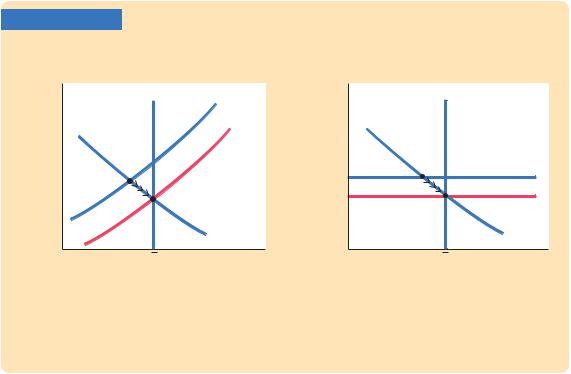
Panel (a) of Figure 11-7 shows the three curves that are necessary for

understanding the short-run and long-run equilibria: the IS curve, the LM

−

curve, and the vertical line representing the natural level of output Y . The LM curve is, as always, drawn for a fixed price level P1. The short-run equilibrium of the economy is point K, where the IS curve crosses the LM curve. Notice that in this short-run equilibrium, the economy’s income is less than its natural level.

Panel (b) of Figure 11-7 shows the same situation in the diagram of aggregate supply and aggregate demand. At the price level P1, the quantity of output demanded is below the natural level. In other words, at the existing price level, there is insufficient demand for goods and services to keep the economy producing at its potential.

In these two diagrams we can examine the short-run equilibrium at which the economy finds itself and the long-run equilibrium toward which the

FIGURE 11-7

The Short-Run and Long-Run Equilibria We can compare the short-run and long-run equilibria using either the IS–LM diagram in panel (a) or the aggregate supply–aggregate demand diagram in panel (b). In the short run, the price level is stuck at P1. The short-run equilibrium of the economy is therefore point K. In the long run, the price level adjusts so that the economy is at the natural level of output. The long-run equilibrium is therefore point C.

C H A P T E R 1 1 Aggregate Demand II: Applying the IS-LM Model | 325

economy gravitates. Point K describes the short-run equilibrium, because it assumes that the price level is stuck at P1. Eventually, the low demand for goods and services causes prices to fall, and the economy moves back toward its natural rate. When the price level reaches P2, the economy is at point C, the long-run equilibrium. The diagram of aggregate supply and aggregate demand shows that at point C, the quantity of goods and services demanded equals the natural level of output. This long-run equilibrium is achieved in the IS –LM diagram by a shift in the LM curve: the fall in the price level raises real money balances and therefore shifts the LM curve to the right.

We can now see the key difference between the Keynesian and classical approaches to the determination of national income. The Keynesian assumption (represented by point K) is that the price level is stuck. Depending on monetary policy, fiscal policy, and the other determinants of aggregate demand, output may deviate from its natural level. The classical assumption (represented by point C) is that the price level is fully flexible. The price level adjusts to ensure that national income is always at its natural level.

To make the same point somewhat differently, we can think of the economy as being described by three equations. The first two are the IS and LM equations:

The IS equation describes the equilibrium in the goods market, and the LM equation describes the equilibrium in the money market. These two equations contain three endogenous variables: Y, P, and r. To complete the system, we need a third equation. The Keynesian approach completes the model with the assumption of fixed prices, so the Keynesian third equation is

P = P1.

This assumption implies that the remaining two variables r and Y must adjust to satisfy the remaining two equations IS and LM. The classical approach completes the model with the assumption that output reaches its natural level, so the classical third equation is

= −

Y Y .

This assumption implies that the remaining two variables r and P must adjust to satisfy the remaining two equations IS and LM. Thus, the classical approach fixes output and allows the price level to adjust to satisfy the goods and money market equilibrium conditions, whereas the Keynesian approach fixes the price level and lets output move to satisfy the equilibrium conditions.

Which assumption is most appropriate? The answer depends on the time horizon. The classical assumption best describes the long run. Hence, our long-run analysis of national income in Chapter 3 and prices in Chapter 4 assumes that output equals its natural level. The Keynesian assumption best describes the short run. Therefore, our analysis of economic fluctuations relies on the assumption of a fixed price level.