C H A P T E R 9 Introduction to Economic Fluctuations | 271

FIGURE 9-6

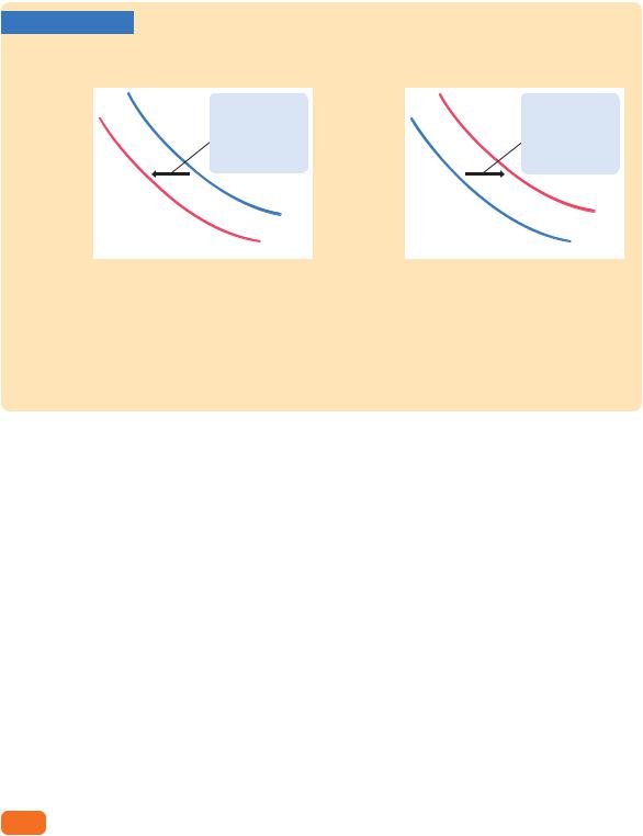
Shifts in the Aggregate Demand Curve Changes in the money supply shift the aggregate demand curve. In panel (a), a decrease in the money supply M reduces the nominal value of output PY. For any given price level P, output Y is lower. Thus, a decrease in the money supply shifts the aggregate demand curve inward from AD1 to AD2. In panel (b), an increase in the money supply M raises the nominal value of output PY. For any given price level P, output Y is higher. Thus, an increase in the money supply shifts the aggregate demand curve outward from AD1 to AD2.

For example, consider what happens if the Fed reduces the money supply. The quantity equation, MV = PY, tells us that the reduction in the money supply leads to a proportionate reduction in the nominal value of output PY. For any given price level, the amount of output is lower, and for any given amount of output, the price level is lower. As in Figure 9-6(a), the aggregate demand curve relating P and Y shifts inward.

The opposite occurs if the Fed increases the money supply. The quantity equation tells us that an increase in M leads to an increase in PY. For any given price level, the amount of output is higher, and for any given amount of output, the price level is higher. As shown in Figure 9-6(b), the aggregate demand curve shifts outward.

Although the quantity theory of money provides a very simple basis for understanding the aggregate demand curve, be forewarned that reality is more complicated. Fluctuations in the money supply are not the only source of fluctuations in aggregate demand. Even if the money supply is held constant, the aggregate demand curve shifts if some event causes a change in the velocity of money. Over the next two chapters, we develop a more general model of aggregate demand, called the IS–LM model, which will allow us to consider many possible reasons for shifts in the aggregate demand curve.

9-4 Aggregate Supply

By itself, the aggregate demand curve does not tell us the price level or the amount of output that will prevail in the economy; it merely gives a relationship between these two variables. To accompany the aggregate demand curve, we

272 | P A R T I V Business Cycle Theory: The Economy in the Short Run

need another relationship between P and Y that crosses the aggregate demand curve—an aggregate supply curve. The aggregate demand and aggregate supply curves together pin down the economy’s price level and quantity of output.

Aggregate supply (AS ) is the relationship between the quantity of goods and services supplied and the price level. Because the firms that supply goods and services have flexible prices in the long run but sticky prices in the short run, the aggregate supply relationship depends on the time horizon. We need to discuss two different aggregate supply curves: the long-run aggregate supply curve LRAS and the short-run aggregate supply curve SRAS. We also need to discuss how the economy makes the transition from the short run to the long run.

The Long Run: The Vertical Aggregate Supply Curve

Because the classical model describes how the economy behaves in the long run, we derive the long-run aggregate supply curve from the classical model. Recall from Chapter 3 that the amount of output produced depends on the fixed amounts of capital and labor and on the available technology. To show this, we write

_ _

Y = F(K, L)

_

= Y .

According to the classical model, output does not depend on the price level. To show that output is fixed at this level, regardless of the price level, we draw a vertical aggregate supply curve, as in Figure 9-7. In the long run, the intersection of

YIncome, output, Y

C H A P T E R 9 Introduction to Economic Fluctuations | 273

the aggregate demand curve with this vertical aggregate supply curve determines the price level.

If the aggregate supply curve is vertical, then changes in aggregate demand affect prices but not output. For example, if the money supply falls, the aggregate demand curve shifts downward, as in Figure 9-8. The economy moves from the old intersection of aggregate supply and aggregate demand, point A, to the new intersection, point B. The shift in aggregate demand affects only prices.

The vertical aggregate supply curve satisfies the classical dichotomy, because it implies that the level of _output is independent of the money supply. This long-run level of output, Y , is called the full-employment, or natural, level of output. It is the level of output at which the economy’s resources are fully employed or, more realistically, at which unemployment is at its natural rate.

The Short Run: The Horizontal Aggregate

Supply Curve

The classical model and the vertical aggregate supply curve apply only in the long run. In the short run, some prices are sticky and, therefore, do not adjust to changes in demand. Because of this price stickiness, the short-run aggregate supply curve is not vertical.

In this chapter, we will simplify things by assuming an extreme example. Suppose that all firms have issued price catalogs and that it is too costly for them to issue new ones. Thus, all prices are stuck at predetermined levels. At these prices, firms are willing to sell as much as their customers are willing to buy, and

274 | P A R T I V Business Cycle Theory: The Economy in the Short Run

Income, output, Y

they hire just enough labor to produce the amount demanded. Because the price level is fixed, we represent this situation in Figure 9-9 with a horizontal aggregate supply curve.

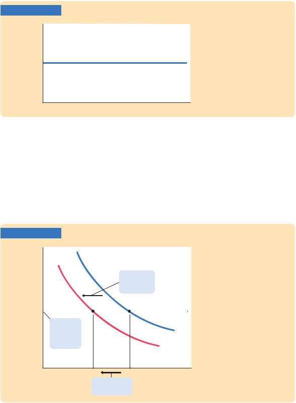
The short-run equilibrium of the economy is the intersection of the aggregate demand curve and this horizontal short-run aggregate supply curve. In this case, changes in aggregate demand do affect the level of output. For example, if the Fed suddenly reduces the money supply, the aggregate demand curve shifts inward, as in Figure 9-10. The economy moves from the old intersection of

Income, output, Y

3. ... lowers the level of output.