


C H A P T E R 7 Economic Growth I: Capital Accumulation and Population Growth | 203
cial circumstances.) The data show a positive relationship between the fraction of output devoted to investment and the level of income per person. That is, countries with high rates of investment, such as the United States and Japan, usually have high incomes, whereas countries with low rates of investment, such as Ethiopia and Burundi, have low incomes. Thus, the data are consistent with the Solow model’s prediction that the investment rate is a key determinant of whether a country is rich or poor.
The strong correlation shown in this figure is an important fact, but it raises as many questions as it resolves. One might naturally ask, why do rates of saving and investment vary so much from country to country? There are many potential answers, such as tax policy, retirement patterns, the development of financial markets, and cultural differences. In addition, political stability may play a role: not surprisingly, rates of saving and investment tend to be low in countries with frequent wars, revolutions, and coups. Saving and investment also tend to be low in countries with poor political institutions, as measured by estimates of official corruption. A final interpretation of the evidence in Figure 7-6 is reverse causation: perhaps high levels of income somehow foster high rates of saving and investment. Unfortunately, there is no consensus among economists about which of the many possible explanations is most important.
The association between investment rates and income per person is strong, and it is an important clue to why some countries are rich and others poor, but it is not the whole story. The correlation between these two variables is far from perfect. The United States and Peru, for instance, have had similar investment rates, but income per person is more than eight times higher in the United States. There must be other determinants of living standards beyond saving and investment. Later in this chapter and also in the next one, we return to the international differences in income per person to see what other variables enter the picture. ■
7-2 The Golden Rule Level of Capital
So far, we have used the Solow model to examine how an economy’s rate of saving and investment determines its steady-state levels of capital and income. This analysis might lead you to think that higher saving is always a good thing because it always leads to greater income. Yet suppose a nation had a saving rate of 100 percent. That would lead to the largest possible capital stock and the largest possible income. But if all of this income is saved and none is ever consumed, what good is it?
This section uses the Solow model to discuss the optimal amount of capital accumulation from the standpoint of economic well-being. In the next chapter, we discuss how government policies influence a nation’s saving rate. But first, in this section, we present the theory behind these policy decisions.

204 | P A R T I I I Growth Theory: The Economy in the Very Long Run
Comparing Steady States
To keep our analysis simple, let’s assume that a policymaker can set the economy’s saving rate at any level. By setting the saving rate, the policymaker determines the economy’s steady state. What steady state should the policymaker choose?
The policymaker’s goal is to maximize the well-being of the individuals who make up the society. Individuals themselves do not care about the amount of capital in the economy, or even the amount of output. They care about the amount of goods and services they can consume. Thus, a benevolent policymaker would want to choose the steady state with the highest level of consumption. The steady-state value of k that maximizes consumption is called the
Golden Rule level of capital and is denoted k* |
.2 |
gold |
|
How can we tell whether an economy is at the Golden Rule level? To answer this question, we must first determine steady-state consumption per worker. Then we can see which steady state provides the most consumption.
To find steady-state consumption per worker, we begin with the national income accounts identity
y = c + i
and rearrange it as
c = y – i.
Consumption is output minus investment. Because we want to find steady-state consumption, we substitute steady-state values for output and investment. Steady-state output per worker is f(k*), where k* is the steady-state capital stock per worker. Furthermore, because the capital stock is not changing in the steady state, investment equals depreciation dk*. Substituting f(k*) for y and dk* for i, we can write steady-state consumption per worker as
c* = f (k*) − dk*.
According to this equation, steady-state consumption is what’s left of steady-state output after paying for steady-state depreciation. This equation shows that an increase in steady-state capital has two opposing effects on steady-state consumption. On the one hand, more capital means more output. On the other hand, more capital also means that more output must be used to replace capital that is wearing out.
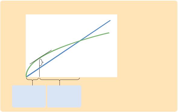
Figure 7-7 graphs steady-state output and steady-state depreciation as a function of the steady-state capital stock. Steady-state consumption is the gap between output and depreciation. This figure shows that there is one level of the
capital stock—the Golden Rule level k* —that maximizes consumption.
gold
When comparing steady states, we must keep in mind that higher levels of capital affect both output and depreciation. If the capital stock is below the
2 Edmund Phelps, “The Golden Rule of Accumulation: A Fable for Growthmen,’’ American Economic Review 51 (September 1961): 638–643.
C H A P T E R 7 Economic Growth I: Capital Accumulation and Population Growth | 205
FIGURE 7-7 |
|
||
Steady-state |
|
|
Steady-state depreciation |
|
|||
output and |
|
|
|
|
|
(and investment), dk* |
|
depreciation |
|
|
|
|
|
|
|
|
|
|
Steady-state |
|
|
|
output, f(k*) |
|
|
|
c* |
|
|
|
gold |
|
|
|
|
Steady-State Consumption
The economy’s output is used for consumption or investment. In the steady state, investment equals depreciation. Therefore, steady-state consumption is the difference between output f ( k *) and depreciation dk*. Steady-state consumption is maximized at the Golden Rule steady state. The Golden Rule capital stock
is denoted k* , and the
gold
Golden Rule level of consump-
tion is denoted c* .
gold
k*
gold
Below the Golden Rule steady state, increases in steady-state capital raise steady-state consumption.
Above the Golden Rule steady state, increases in steady-state capital reduce steady-state consumption.
Steady-state capital per worker, k*
Golden Rule level, an increase in the capital stock raises output more than depreciation, so consumption rises. In this case, the production function is steeper than the dk* line, so the gap between these two curves—which equals consumption—grows as k* rises. By contrast, if the capital stock is above the Golden Rule level, an increase in the capital stock reduces consumption, because the increase in output is smaller than the increase in depreciation. In this case, the production function is flatter than the dk* line, so the gap between the curves—consumption—shrinks as k* rises. At the Golden Rule level of capital, the production function and the dk* line have the same slope, and consumption is at its greatest level.
We can now derive a simple condition that characterizes the Golden Rule level of capital. Recall that the slope of the production function is the marginal product of capital MPK. The slope of the dk* line is d. Because these two slopes are equal at k*gold, the Golden Rule is described by the equation
MPK = d.
At the Golden Rule level of capital, the marginal product of capital equals the depreciation rate.
To make the point somewhat differently, suppose that the economy starts at some steady-state capital stock k* and that the policymaker is considering increasing the capital stock to k* + 1. The amount of extra output from this increase in capital would be f(k* + 1) – f(k*), the marginal product of capital MPK. The amount of extra depreciation from having 1 more unit of capital is
206 | P A R T I I I Growth Theory: The Economy in the Very Long Run
the depreciation rate d. Thus, the net effect of this extra unit of capital on consumption is MPK – d. If MPK – d > 0, then increases in capital increase consumption, so k* must be below the Golden Rule level. If MPK – d < 0, then increases in capital decrease consumption, so k* must be above the Golden Rule level. Therefore, the following condition describes the Golden Rule:
MPK − d = 0.
At the Golden Rule level of capital, the marginal product of capital net of depreciation (MPK – d) equals zero. As we will see, a policymaker can use this condition to find the Golden Rule capital stock for an economy.3
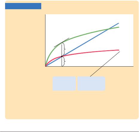
Keep in mind that the economy does not automatically gravitate toward the Golden Rule steady state. If we want any particular steady-state capital stock, such as the Golden Rule, we need a particular saving rate to support it. Figure 7-8 shows the steady state if the saving rate is set to produce the Golden Rule level of capital. If the saving rate is higher than the one used in this figure, the
FIGURE 7-8
Steady-state output, depreciation, and investment per worker
|
dk* |
|
f(k*) |
c* |
sgold f(k*) |
gold |
|
i* |
|
gold |
|
k* |
Steady-state capital |
|
gold |
per worker, k* |
|
|
|
|
|
|
|
1. To reach the Golden Rule steady state ...
2. ...the economy needs the right saving rate.
The Saving Rate and the Golden Rule There is only one saving rate that produces the Golden Rule level of
capital k* . Any change in the saving rate would shift
gold
the sf (k) curve and would move the economy to a steady state with a lower level of consumption.
3 Mathematical note: Another way to derive the condition for the Golden Rule uses a bit of calculus. Recall that c * = f(k*) − dk*. To find the k* that maximizes c *, differentiate to find dc */dk* = f ′(k*) − d and set this derivative equal to zero. Noting that f ′(k*) is the marginal product of capital, we obtain the Golden Rule condition in the text.

C H A P T E R 7 Economic Growth I: Capital Accumulation and Population Growth | 207
steady-state capital stock will be too high. If the saving rate is lower, the steadystate capital stock will be too low. In either case, steady-state consumption will be lower than it is at the Golden Rule steady state.
Finding the Golden Rule Steady State:
A Numerical Example
Consider the decision of a policymaker choosing a steady state in the following economy. The production function is the same as in our earlier example:
y = k.
Output per worker is the square root of capital per worker. Depreciation d is again 10 percent of capital. This time, the policymaker chooses the saving rate s and thus the economy’s steady state.
To see the outcomes available to the policymaker, recall that the following equation holds in the steady state:
k* s
= . f(k*) d
In this economy, this equation becomes
k* s
= .
k* 0.1
Squaring both sides of this equation yields a solution for the steady-state capital stock. We find
k* = 100s 2.
Using this result, we can compute the steady-state capital stock for any saving rate. Table 7-3 presents calculations showing the steady states that result from various saving rates in this economy. We see that higher saving leads to a higher capital stock, which in turn leads to higher output and higher depreciation. Steady-state consumption, the difference between output and depreciation, first rises with higher saving rates and then declines. Consumption is highest when the saving rate is 0.5. Hence, a saving rate of 0.5 produces the Golden Rule
steady state.
Recall that another way to identify the Golden Rule steady state is to find the capital stock at which the net marginal product of capital (MPK – d) equals zero. For this production function, the marginal product is4
1
MPK = . 2 k
4 Mathematical note: To derive this formula, note that the marginal product of capital is the derivative of the production function with respect to k.