

C H A P T E R 5 The Open Economy | 161
FIGURE 5-23
(a) The Market for Loanable Funds
Real interest rate, r
2. ...
causes the
interest
rate to
fall, ...
S
1. A fall in net
capital outflow ...
I + CF
Loanable funds, S, I + CF
(b) Net Capital Outflow
r
r1
r2
|
|
CF(r) |
|
|
|
CF2 |
CF1 |
Net capital |
|
|
outflow, CF |
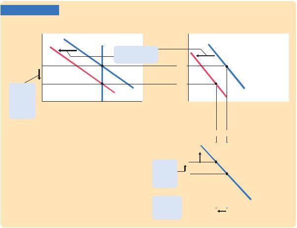
A Fall in the Net Capital Outflow in the Large Open Economy Panel (a) shows that a downward shift in the CF schedule reduces the demand for loans and thereby reduces the equilibrium interest rate. Panel (b) shows that the level of the net capital outflow falls. Panel (c) shows that the real exchange rate appreciates, and net exports fall.
|
|
|
(c) The Market for Foreign Exchange |
||||
Real |
|
|
|
|
|
|
|
|
e2 |
|
|
|
|
||
exchange |
|
|
CF |
|
|||
rate, e |
e2 |
|
|
|
|
||
3. ... the |
e1 |
|
|
|
|
||
|
|
|
|
|
|||
exchange |
e1 |
|
|
|
|
|
|
rate to |
|
|
|
|
|
||
rise, ... |
|
|
|
|
|
|
|
4. ... and |
|
|
|
|
|
NX(e) |
|
net exports |
|
|
|
|
|
|
|
|
NX2 |
|
NX1 |
Net exports, NX |
|||
to fall. |
|
|
|
||||
mitigates the shift in the CF schedule, CF still falls. The reduced level of net capital outflow reduces the supply of dollars in the market for foreign exchange. The exchange rate appreciates, and net exports fall.
Conclusion
How different are large and small open economies? Certainly, policies affect the interest rate in a large open economy, unlike in a small open economy. But, in other ways, the two models yield similar conclusions. In both large and small open economies, policies that raise saving or lower investment lead to trade surpluses. Similarly, policies that lower saving or raise investment lead to trade deficits. In both economies, protectionist trade policies cause the exchange rate to appreciate and do not influence the trade balance. Because the results are so similar, for most questions one can use the simpler model of the small open economy, even if the economy being examined is not really small.
162 | P A R T I I Classical Theory: The Economy in the Long Run
M O R E P R O B L E M S A N D A P P L I C A T I O N S
1.If a war broke out abroad, it would affect the U.S. economy in many ways. Use the model of the large open economy to examine each of the following effects of such a war. What happens in the United States to saving, investment, the trade balance, the interest rate, and the exchange rate? (To keep things simple, consider each of the following effects separately.)
a.The U.S. government, fearing it may need to enter the war, increases its purchases of military equipment.
b.Other countries raise their demand for high-tech weapons, a major export of the United States.
c.The war makes U.S. firms uncertain about the future, and the firms delay some investment projects.
d.The war makes U.S. consumers uncertain about the future, and the consumers save more in response.
e. Americans become apprehensive about traveling abroad, so more of them spend their vacations in the United States.
f. Foreign investors seek a safe haven for their portfolios in the United States.
2.On September 21, 1995, “House Speaker Newt Gingrich threatened to send the United States into default on its debt for the first time in the nation’s history, to force the Clinton Administration to balance the budget on Republican terms” (New York Times, September 22, 1995,
p. A1). That same day, the interest rate on
30-year U.S. government bonds rose from 6.46 to 6.55 percent, and the dollar fell in value from 102.7 to 99.0 yen. Use the model of the large open economy to explain this event.

C H A P T E R 6
Unemployment
A man willing to work, and unable to find work, is perhaps the saddest sight
that fortune’s inequality exhibits under the sun.
—Thomas Carlyle
Unemployment is the macroeconomic problem that affects people most directly and severely. For most people, the loss of a job means a reduced living standard and psychological distress. It is no surprise that unem-
ployment is a frequent topic of political debate and that politicians often claim that their proposed policies would help create jobs.
Economists study unemployment to identify its causes and to help improve the public policies that affect the unemployed. Some of these policies, such as job-training programs, help people find employment. Others, such as unemployment insurance, alleviate some of the hardships that the unemployed face. Still other policies affect the prevalence of unemployment inadvertently. Laws mandating a high minimum wage, for instance, are widely thought to raise unemployment among the least skilled and experienced members of the labor force.
Our discussions of the labor market so far have ignored unemployment. In particular, the model of national income in Chapter 3 was built with the assumption that the economy is always at full employment. In reality, not everyone in the labor force has a job all the time: in all free-market economies, at any moment, some people are unemployed.
Figure 6-1 shows the rate of unemployment—the percentage of the labor force unemployed—in the United States since 1950. Although the rate of unemployment fluctuates from year to year, it never gets even close to zero. The average is between 5 and 6 percent, meaning that about 1 out of every 18 people wanting a job does not have one.
In this chapter we begin our study of unemployment by discussing why there is always some unemployment and what determines its level. We do not study what determines the year-to-year fluctuations in the rate of unemployment until Part Four of this book, which examines short-run economic fluctuations. Here we examine the determinants of the natural rate of unemployment—the average rate of unemployment around which the
163

164 | P A R T I I Classical Theory: The Economy in the Long Run
FIGURE 6-1 |
|
|
|
|
|
|
|
|
|
|
|
|
Percent |
12 |
|
|
|
Unemployment rate |
|
|
|
|
|
|
|
unemployed |
|
|
|
|
|
|
|
|
|
|
||
|
10 |
|
|
|
|
|
|
|
|
|
|
|
|
8 |
|
|
|
|
|
|
|
|
|
|
|
|
6 |
|
|
|
|
|
|
|
|
|
|
|
|
4 |
|
|
|
|
|
|
Natural rate |
|
|
|
|
|
|
|
|
|
|
|
of unemployment |
|
|
|
||
|
|
|
|
|
|
|
|
|
|
|
||
|
2 |
|
|
|
|
|
|
|
|
|
|
|
|
0 |
|
|
|
|
|
|
|
|
|
|
|
|
1950 |
1955 |
1960 |
1965 |
1970 |
1975 |
1980 |
1985 |
1990 |
1995 |
2000 |
2005 |
|
|
|
|
|
|
|
|
|
|
|
|
Year |
The Unemployment Rate and the Natural Rate of Unemployment in the United States There is always some unemployment. The natural rate of unemployment is the average level around which the unemployment rate fluctuates. (The natural rate of unemployment for any particular month is estimated here by averaging all the unemployment rates from ten years earlier to ten years later. Future unemployment rates are set at 5.5 percent.)
Source: Bureau of Labor Statistics.
economy fluctuates. The natural rate is the rate of unemployment toward which the economy gravitates in the long run, given all the labor-market imperfections that impede workers from instantly finding jobs.
6-1 Job Loss, Job Finding, and the
Natural Rate of Unemployment
Every day some workers lose or quit their jobs, and some unemployed workers are hired. This perpetual ebb and flow determines the fraction of the labor force that is unemployed. In this section we develop a model of labor-force dynamics that shows what determines the natural rate of unemployment.1
1 Robert E. Hall, “A Theory of the Natural Rate of Unemployment and the Duration of Unemployment,” Journal of Monetary Economics 5 (April 1979): 153–169.
C H A P T E R 6 Unemployment | 165
We start with some notation. Let L denote the labor force, E the number of employed workers, and U the number of unemployed workers. Because every worker is either employed or unemployed, the labor force is the sum of the employed and the unemployed:
L = E + U.
In this notation, the rate of unemployment is U/L.
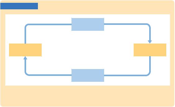
To see what factors determine the unemployment rate, we assume that the labor force L is fixed and focus on the transition of individuals in the labor force between employment E and unemployment U. This is illustrated in Figure 6-2. Let s denote the rate of job separation, the fraction of employed individuals who lose or leave their job each month. Let f denote the rate of job finding, the fraction of unemployed individuals who find a job each month. Together, the rate of job separation s and the rate of job finding f determine the rate of unemployment.
If the unemployment rate is neither rising nor falling—that is, if the labor market is in a steady state—then the number of people finding jobs fU must equal the number of people losing jobs sE. We can write the steady-state condition as
f U = sE.
We can use this equation to find the steady-state unemployment rate. From our definition of the labor force, we know that E = L − U; that is, the number of employed equals the labor force minus the number of unemployed. If we substitute (L − U ) for E in the steady-state condition, we find
f U = s(L − U ).
FIGURE 6-2
Job Separation (s)
Employed |
Unemployed |
Job Finding (f)
The Transitions Between Employment and Unemployment In every period, a fraction s of the employed lose their jobs, and a fraction f of the unemployed find jobs. The rates of job separation and job finding determine the rate of unemployment.

166 | P A R T I I Classical Theory: The Economy in the Long Run
Next, we divide both sides of this equation by L to obtain
f U = s(1 − U ).
L |
|
L |
||||||
Now we can solve for U/L to find |
|
|
|
|
||||
|
|
U |
= |
|
s |
. |
||
|
|
L |
|
s + f |
||||
This can also be written as |
|
|
|
|
||||
|
U |
= |
1 |
|
. |
|||
|
L |
1+ f/s |
||||||
This equation shows that the steady-state rate of unemployment U/L depends on the rates of job separation s and job finding f. The higher the rate of job separation, the higher the unemployment rate. The higher the rate of job finding, the lower the unemployment rate.
Here’s a numerical example. Suppose that 1 percent of the employed lose their jobs each month (s = 0.01). This means that on average jobs last 100 months, or about 8 years. Suppose further that 20 percent of the unemployed find a job each month ( f = 0.20), so that spells of unemployment last 5 months on average. Then the steady-state rate of unemployment is
U |
= |
0.01 |
|
L |
0.01 + |
0.20 |
|
= 0.0476. |
|
||
The rate of unemployment in this example is about 5 percent.
This simple model of the natural rate of unemployment has an important implication for public policy. Any policy aimed at lowering the natural rate of unemployment must either reduce the rate of job separation or increase the rate of job finding. Similarly, any policy that affects the rate of job separation or job finding also changes the natural rate of unemployment.
Although this model is useful in relating the unemployment rate to job separation and job finding, it fails to answer a central question: why is there unemployment in the first place? If a person could always find a job quickly, then the rate of job finding would be very high and the rate of unemployment would be near zero. This model of the unemployment rate assumes that job finding is not instantaneous, but it fails to explain why. In the next two sections, we examine two underlying reasons for unemployment: job search and wage rigidity.
6-2 Job Search and Frictional
Unemployment
One reason for unemployment is that it takes time to match workers and jobs. The equilibrium model of the aggregate labor market discussed in Chapter 3 assumes that all workers and all jobs are identical and, therefore, that all workers