

68 | P A R T I I Classical Theory: The Economy in the Long Run
FIGURE 3-8
Real interest rate, r
Saving , S
Equilibrium interest rate
Desired investment, I(r)
S |
Investment, Saving, I, S |
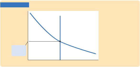
Saving, Investment, and the Interest Rate The interest rate adjusts to bring saving and investment into balance. The vertical line represents saving—the supply of loanable funds. The downward-sloping line represents investment— the demand for loanable funds. The intersection of these two curves determines the equilibrium interest rate.
“price” is the interest rate. Saving is the supply of loanable funds—households lend their saving to investors or deposit their saving in a bank that then loans the funds out. Investment is the demand for loanable funds—investors borrow from the public directly by selling bonds or indirectly by borrowing from banks. Because investment depends on the interest rate, the quantity of loanable funds demanded also depends on the interest rate.
The interest rate adjusts until the amount that firms want to invest equals the amount that households want to save. If the interest rate is too low, investors want more of the economy’s output than households want to save. Equivalently, the quantity of loanable funds demanded exceeds the quantity supplied. When this happens, the interest rate rises. Conversely, if the interest rate is too high, households want to save more than firms want to invest; because the quantity of loanable funds supplied is greater than the quantity demanded, the interest rate falls. The equilibrium interest rate is found where the two curves cross. At the equilibrium interest rate, households’ desire to save balances firms’ desire to invest, and the quantity of loanable funds supplied equals the quantity demanded.
Changes in Saving: The Effects of Fiscal Policy
We can use our model to show how fiscal policy affects the economy. When the government changes its spending or the level of taxes, it affects the demand for the economy’s output of goods and services and alters national saving, investment, and the equilibrium interest rate.
An Increase in Government Purchases Consider first the effects of an
increase in government purchases by an amount |
G. The immediate impact is to |
increase the demand for goods and services by |
G. But because total output is |
fixed by the factors of production, the increase in government purchases must be met by a decrease in some other category of demand. Disposable income Y − T

C H A P T E R 3 National Income: Where It Comes From and Where It Goes | 69
FYI
The Financial System: Markets, Intermediaries,
and the Crisis of 2008–2009
The model presented in this chapter represents the economy’s financial system with a single market—the market for loanable funds. Those who have some income they don’t want to consume immediately bring their saving to this market. Those who have investment projects they want to undertake finance them by borrowing in this market. The interest rate adjusts to bring saving and investment into balance.
The actual financial system is a bit more complicated than this description. As in this model, the goal of the system is to channel resources from savers into various forms of investment. But the system includes a large variety of mechanisms to facilitate this transfer of resources.
One piece of the financial system is the set of financial markets through which households can directly provide resources for investment. Two important financial markets are the market for bonds and the market for stocks. A person who buys a bond from, say, Apple Corporation becomes a creditor of the company, while a person who buys newly issued stock from Apple becomes a part owner of the company. (A purchase of stock on a stock exchange, however, represents a transfer of ownership shares from one person to another and does not provide new funds for investment projects.) Raising investment funds by issuing bonds is called debt finance, and raising funds by issuing stock is called equity finance.
Another piece of the financial system is the set of financial intermediaries through which households can indirectly provide resources for investment. As the term suggests, a financial intermediary stands
between the two sides of the market and helps direct financial resources toward their best use. Banks are the best-known type of financial intermediary. They take deposits from savers and use these deposits to make loans to those who have investments to make. Other examples of financial intermediaries include mutual funds, pension funds, and insurance companies. Unlike in financial markets, when a financial intermediary is involved, the saver is often unaware of the investments that his saving is financing.
In 2008 and 2009, the world financial system experienced a historic crisis. Many banks and other financial intermediaries had previously made loans to homeowners, called mortgages, and had purchased many mortgage-backed securities (financial instruments whose value derives from a pool of mortgages). A large decline in housing prices throughout the United States, however, caused many homeowners to default on their mortgages, which in turn led to large losses at these financial institutions. Many banks and other financial intermediaries found themselves nearly bankrupt, and the financial system started having trouble performing its key functions. To address the problem, the U.S. Congress in October 2008 authorized the U.S. Treasury to spend $700 billion, which was largely used to put further resources into the banking system.
In Chapter 11 we will examine more fully the financial crisis of 2008 and 2009. For our purposes in this chapter, and as a building block for further analysis, representing the entire financial system by a single market for loanable funds is a useful simplification.
is unchanged, so consumption C is unchanged as well. Therefore, the increase in government purchases must be met by an equal decrease in investment.
To induce investment to fall, the interest rate must rise. Hence, the increase in government purchases causes the interest rate to increase and investment to decrease. Government purchases are said to crowd out investment.
To grasp the effects of an increase in government purchases, consider the impact on the market for loanable funds. Because the increase in government purchases is not accompanied by an increase in taxes, the government finances the additional spending by borrowing—that is, by reducing public saving. With

70 | P A R T I I Classical Theory: The Economy in the Long Run
FIGURE 3-9
Real interest rate, r |
S2 |
|
S1 |
|
|
|
|
||
|
|
|
|
|
|
|
|
|
|
|
|
|
1. A fall in |
|
r2 |
|
saving ... |
||
|
|
|
||
|
|
2. ... raises |
|
|
|
|
the interest |
|
|
|
|
|
|
|
r1 |
rate. |
|
|
|
|
|
|
||
I(r)
Investment, Saving, I, S
A Reduction in Saving A reduction in saving, possibly the result of a change in fiscal policy, shifts the saving schedule to the left. The new equilibrium is the point at which the new saving schedule crosses the investment schedule. A reduction in saving lowers the amount of investment and raises the interest rate. Fiscal-policy actions that reduce saving are said to crowd out investment.
private saving unchanged, this government borrowing reduces national saving. As Figure 3-9 shows, a reduction in national saving is represented by a leftward shift in the supply of loanable funds available for investment. At the initial interest rate, the demand for loanable funds exceeds the supply. The equilibrium interest rate rises to the point where the investment schedule crosses the new saving schedule. Thus, an increase in government purchases causes the interest rate to rise from r1 to r2.
CASE STUDY
Wars and Interest Rates in the United Kingdom, 1730–1920
Wars are traumatic—both for those who fight them and for a nation’s economy. Because the economic changes accompanying them are often large, wars provide a natural experiment with which economists can test their theories. We can learn about the economy by seeing how in wartime the endogenous variables respond to the major changes in the exogenous variables.
One exogenous variable that changes substantially in wartime is the level of government purchases. Figure 3-10 shows military spending as a percentage of GDP for the United Kingdom from 1730 to 1919. This graph shows, as one would expect, that government purchases rose suddenly and dramatically during the eight wars of this period.
Our model predicts that this wartime increase in government purchases—and the increase in government borrowing to finance the wars—should have raised the demand for goods and services, reduced the supply of loanable funds, and raised the interest rate. To test this prediction, Figure 3-10 also shows the interest rate on long-term government bonds, called consols in the United Kingdom. A positive association between military purchases and interest rates is apparent in

C H A P T E R 3 National Income: Where It Comes From and Where It Goes | 71
FIGURE 3-10
Percentage |
|
|
|
|
|
|
|
|
|
Interest rate |
of GDP |
|
|
|
|
|
|
|
|
|
(percent) |
50 |
|
|
|
|
|
|
|
|
|
6 |
|
|
|
|
|
|
|
|
|
|
World |
45 |
|
|
|
|
|
Interest rates |
|
|
War I |
|
|
|
|
|
|
|
|
|
5 |
||
40 |
|
|
|
|
|
(right scale) |
|
|
||
|
|
|
|
|
|
|
|
|
|
|
35 |
|
|
|
|
|
|
|
|
|
4 |
|
|
|
|
|
|
|
|
|
|
|
30 |
|
|
|
|
|
|
|
|
|
|
25 |
|
|
|
|
|
|
|
|
|
3 |
20 |
|
War of |
War of American |
|
|
|
|
|
||
15 |
|
Austrian |
Independence |
|
|
Military spending |
2 |
|||
Succession |
|
Wars with France |
|
|||||||
10 |
|
Seven Years War |
|
|
|
(left scale) |
Boer War |
|||
|
|
|
|
|
|
|||||
|
|
|
|
|
|
|
|
|||
|
|
|
|
|
|
Crimean War |
|
1 |
||
|
|
|
|
|
|
|
|
|||
|
|
|
|
|
|
|
|
|
||
5 |
|
|
|
|
|
|
|
|
|
|
0 |
|
1750 |
1770 |
1790 |
1810 |
1830 |
1850 |
1870 |
1890 |
0 |
1730 |
1910 |
|||||||||
Year
Military Spending and the Interest Rate in the United Kingdom This figure shows military spending as a percentage of GDP in the United Kingdom from 1730 to 1919. Not surprisingly, military spending rose substantially during each of the eight wars of this period. This figure also shows that the interest rate tended to rise when military spending rose.
Source: Series constructed from various sources described in Robert J. Barro, “Government Spending, Interest Rates, Prices, and Budget Deficits in the United Kingdom, 1701–1918,” Journal of Monetary Economics 20 (September 1987): 221–248.
this figure. These data support the model’s prediction: interest rates do tend to rise when government purchases increase.7
One problem with using wars to test theories is that many economic changes may be occurring at the same time. For example, in World War II, while government purchases increased dramatically, rationing also restricted consumption of many goods. In addition, the risk of defeat in the war and default by the government on its debt presumably increases the interest rate the government must pay. Economic models predict what happens when one exogenous variable changes and all the other exogenous variables remain constant. In the real world,
7 Daniel K. Benjamin and Levis A. Kochin,“War, Prices, and Interest Rates: A Martial Solution to Gibson’s Paradox,” in M. D. Bordo and A. J. Schwartz, eds., A Retrospective on the Classical Gold Standard, 1821−1931 (Chicago: University of Chicago Press, 1984), 587– 612; Robert J. Barro, “Government Spending, Interest Rates, Prices, and Budget Deficits in the United Kingdom, 1701–1918,” Journal of Monetary Economics 20 (September 1987): 221–248.