390 | P A R T I V Business Cycle Theory: The Economy in the Short Run

when we are studying unemployment and inflation. But we should not lose sight of the fact that the Phillips curve and the aggregate supply curve are two sides of the same coin.

Adaptive Expectations and Inflation Inertia

To make the Phillips curve useful for analyzing the choices facing policymakers, we need to specify what determines expected inflation. A simple and often plausible assumption is that people form their expectations of inflation based on recently observed inflation. This assumption is called adaptive expectations. For example, suppose that people expect prices to rise this year at the same rate as they did last year. Then expected inflation Ep equals last year’s inflation p−1:

Ep = p−1

In this case, we can write the Phillips curve as

p = p−1 − b(u − un) + u,

which states that inflation depends on past inflation, cyclical unemployment, and a supply shock. When the Phillips curve is written in this form, the natural rate of unemployment is sometimes called the non-accelerating inflation rate of unemployment, or NAIRU.

The first term in this form of the Phillips curve, p−1, implies that inflation has inertia. That is, like an object moving through space, inflation keeps going unless something acts to stop it. In particular, if unemployment is at the NAIRU and if

7 A. W. Phillips, “The Relationship Between Unemployment and the Rate of Change of Money Wages in the United Kingdom, 1861–1957,” Economica 25 (November 1958): 283–299.

C H A P T E R 1 3 Aggregate Supply and the Short-Run Tradeoff Between Inflation and Unemployment | 391

there are no supply shocks, the continued rise in price level neither speeds up nor slows down. This inertia arises because past inflation influences expectations of future inflation and because these expectations influence the wages and prices that people set. Robert Solow captured the concept of inflation inertia well when, during the high inflation of the 1970s, he wrote,“Why is our money ever less valuable? Perhaps it is simply that we have inflation because we expect inflation, and we expect inflation because we’ve had it.’’

In the model of aggregate supply and aggregate demand, inflation inertia is interpreted as persistent upward shifts in both the aggregate supply curve and the aggregate demand curve. First, consider aggregate supply. If prices have been rising quickly, people will expect them to continue to rise quickly. Because the position of the short-run aggregate supply curve depends on the expected price level, the short-run aggregate supply curve will shift upward over time. It will continue to shift upward until some event, such as a recession or a supply shock, changes inflation and thereby changes expectations of inflation.

The aggregate demand curve must also shift upward to confirm the expectations of inflation. Most often, the continued rise in aggregate demand is due to persistent growth in the money supply. If the Fed suddenly halted money growth, aggregate demand would stabilize, and the upward shift in aggregate supply would cause a recession. The high unemployment in the recession would reduce inflation and expected inflation, causing inflation inertia to subside.

Two Causes of Rising and Falling Inflation

The second and third terms in the Phillips curve equation show the two forces that can change the rate of inflation.

The second term, b(u − un), shows that cyclical unemployment—the deviation of unemployment from its natural rate—exerts upward or downward pressure on inflation. Low unemployment pulls the inflation rate up. This is called demand-pull inflation because high aggregate demand is responsible for this type of inflation. High unemployment pulls the inflation rate down. The parameter b measures how responsive inflation is to cyclical unemployment.

The third term, u, shows that inflation also rises and falls because of supply shocks. An adverse supply shock, such as the rise in world oil prices in the 1970s, implies a positive value of u and causes inflation to rise. This is called cost-push inflation because adverse supply shocks are typically events that push up the costs of production. A beneficial supply shock, such as the oil glut that led to a fall in oil prices in the 1980s, makes u negative and causes inflation to fall.

CASE STUDY

Inflation and Unemployment in the United States

Because inflation and unemployment are such important measures of economic performance, macroeconomic developments are often viewed through the lens of the Phillips curve. Figure 13-3 displays the history of inflation and

392 | P A R T I V Business Cycle Theory: The Economy in the Short Run

Unemployment (percent)

Inflation and Unemployment in the United States, 1960–2008 This figure uses annual data on the unemployment rate and the inflation rate (percentage change in the GDP deflator) to illustrate macroeconomic developments spanning almost half a century of U.S. history.

Source: U.S. Department of Commerce and U.S. Department of Labor.

unemployment in the United States from 1960 to 2008. This data, spanning almost half a century, illustrates some of the causes of rising or falling inflation.

The 1960s showed how policymakers can, in the short run, lower unemployment at the cost of higher inflation. The tax cut of 1964, together with expansionary monetary policy, expanded aggregate demand and pushed the unemployment rate below 5 percent. This expansion of aggregate demand continued in the late 1960s largely as a by-product of government spending for the Vietnam War. Unemployment fell lower and inflation rose higher than policymakers intended.

The 1970s were a period of economic turmoil. The decade began with policymakers trying to lower the inflation inherited from the 1960s. President Nixon imposed temporary controls on wages and prices, and the Federal Reserve engineered a recession through contractionary monetary policy, but the inflation rate fell only slightly. The effects of wage and price controls ended when the controls were lifted, and the recession was too small to counteract the inflationary impact of the boom that had preceded it. By 1972 the unemployment rate was the same as a decade earlier, while inflation was 3 percentage points higher.

Beginning in 1973 policymakers had to cope with the large supply shocks caused by the Organization of Petroleum Exporting Countries (OPEC). OPEC

C H A P T E R 1 3 Aggregate Supply and the Short-Run Tradeoff Between Inflation and Unemployment | 393

first raised oil prices in the mid-1970s, pushing the inflation rate up to about 10 percent. This adverse supply shock, together with temporarily tight monetary policy, led to a recession in 1975. High unemployment during the recession reduced inflation somewhat, but further OPEC price hikes pushed inflation up again in the late 1970s.

The 1980s began with high inflation and high expectations of inflation. Under the leadership of Chairman Paul Volcker, the Federal Reserve doggedly pursued monetary policies aimed at reducing inflation. In 1982 and 1983 the unemployment rate reached its highest level in 40 years. High unemployment, aided by a fall in oil prices in 1986, pulled the inflation rate down from about 10 percent to about 3 percent. By 1987 the unemployment rate of about 6 percent was close to most estimates of the natural rate. Unemployment continued to fall through the 1980s, however, reaching a low of 5.2 percent in 1989 and beginning a new round of demand-pull inflation.

Compared to the preceding 30 years, the 1990s and early 2000s were relatively quiet. The 1990s began with a recession caused by several contractionary shocks to aggregate demand: tight monetary policy, the savings-and-loan crisis, and a fall in consumer confidence coinciding with the Gulf War. The unemployment rate rose to 7.3 percent in 1992, and inflation fell slightly. Unlike in the 1982 recession, unemployment in the 1990 recession was never far above the natural rate, so the effect on inflation was small. Similarly, a recession in 2001 (discussed in Chapter 11) raised unemployment, but the downturn was mild by historical standards, and the impact on inflation was once again slight. A more severe recession beginning in 2008 (also discussed in Chapter 11) looked like it might put more significant downward pressure on inflation—although the full magnitude of this event was uncertain as this book was going to press.

Thus, U.S. macroeconomic history exhibits the two causes of changes in the inflation rate that we encountered in the Phillips curve equation. The 1960s and 1980s show the two sides of demand-pull inflation: in the 1960s low unemployment pulled inflation up, and in the 1980s high unemployment pulled inflation down. The oil-price hikes of the 1970s show the effects of cost-push inflation. ■

The Short-Run Tradeoff Between Inflation

and Unemployment

Consider the options the Phillips curve gives to a policymaker who can influence aggregate demand with monetary or fiscal policy. At any moment, expected inflation and supply shocks are beyond the policymaker’s immediate control. Yet, by changing aggregate demand, the policymaker can alter output, unemployment, and inflation. The policymaker can expand aggregate demand to lower unemployment and raise inflation. Or the policymaker can depress aggregate demand to raise unemployment and lower inflation.

Figure 13-4 plots the Phillips curve equation and shows the short-run tradeoff between inflation and unemployment. When unemployment is at its natural rate (u = un), inflation depends on expected inflation and the supply shock (p = Ep + u). The parameter b determines the slope of the tradeoff between inflation

394 | P A R T I V Business Cycle Theory: The Economy in the Short Run

FIGURE 13-4

and unemployment. In the short run, for a given level of expected inflation, policymakers can manipulate aggregate demand to choose any combination of inflation and unemployment on this curve, called the short-run Phillips curve.

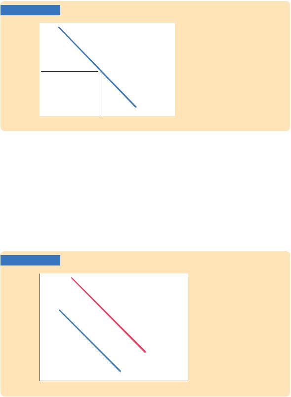
Notice that the position of the short-run Phillips curve depends on the expected rate of inflation. If expected inflation rises, the curve shifts upward, and the policymaker’s tradeoff becomes less favorable: inflation is higher for any level of unemployment. Figure 13-5 shows how the tradeoff depends on expected inflation.

Because people adjust their expectations of inflation over time, the tradeoff between inflation and unemployment holds only in the short run. The