C H A P T E R 1 2 The Open Economy Revisited: The Mundell-Fleming Model and the Exchange-Rate Regime | 375

Fiscal Policy

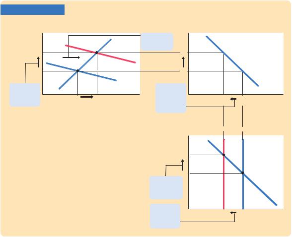
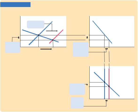
Figure 12-16 examines the impact of a fiscal expansion. An increase in government purchases or a cut in taxes shifts the IS curve to the right. As panel (a) illustrates, this shift in the IS curve leads to an increase in the level of income and an increase in the interest rate. These two effects are similar to those in a closed economy.

Yet, in the large open economy, the higher interest rate reduces the net capital outflow, as in panel (b). The fall in the net capital outflow reduces the supply of dollars in the market for foreign exchange. The exchange rate appreciates, as in panel (c). Because domestic goods become more expensive relative to foreign goods, net exports fall.

Figure 12-16 shows that a fiscal expansion does raise income in the large open economy, unlike in a small open economy under a floating exchange rate. The impact on income, however, is smaller than in a closed economy. In a closed economy, the expansionary impact of fiscal policy is partially offset by the crowding out of investment: as the interest rate rises, investment falls, reducing

FIGURE 12-16

376 | P A R T I V Business Cycle Theory: The Economy in the Short Run

the fiscal-policy multipliers. In a large open economy, there is yet another offsetting factor: as the interest rate rises, the net capital outflow falls, the currency appreciates in the foreign-exchange market, and net exports fall. Together these effects are not large enough to make fiscal policy powerless, as it is in a small open economy, but they do reduce the impact of fiscal policy.

Monetary Policy

Figure 12-17 examines the effect of a monetary expansion. An increase in the money supply shifts the LM curve to the right, as in panel (a). The level of income rises, and the interest rate falls. Once again, these effects are similar to those in a closed economy.

Yet, as panel (b) shows, the lower interest rate leads to a higher net capital outflow. The increase in CF raises the supply of dollars in the market for foreign exchange. The exchange rate falls, as in panel (c). As domestic goods become cheaper relative to foreign goods, net exports rise.

FIGURE 12-17

C H A P T E R 1 2 The Open Economy Revisited: The Mundell-Fleming Model and the Exchange-Rate Regime | 377

We can now see that the monetary transmission mechanism works through two channels in a large open economy. As in a closed economy, a monetary expansion lowers the interest rate, which stimulates investment. As in a small open economy, a monetary expansion causes the currency to depreciate in the market for foreign exchange, which stimulates net exports. Both effects result in a higher level of aggregate income.

A Rule of Thumb

This model of the large open economy describes well the U.S. economy today. Yet it is somewhat more complicated and cumbersome than the model of the closed economy we studied in Chapters 10 and 11 and the model of the small open economy we developed in this chapter. Fortunately, there is a useful rule of thumb to help you determine how policies influence a large open economy without remembering all the details of the model: The large open economy is an average of the closed economy and the small open economy.To find how any policy will affect any variable, find the answer in the two extreme cases and take an average.

For example, how does a monetary contraction affect the interest rate and investment in the short run? In a closed economy, the interest rate rises, and investment falls. In a small open economy, neither the interest rate nor investment changes. The effect in the large open economy is an average of these two cases: a monetary contraction raises the interest rate and reduces investment, but only somewhat. The fall in the net capital outflow mitigates the rise in the interest rate and the fall in investment that would occur in a closed economy. But unlike in a small open economy, the international flow of capital is not so strong as to negate fully these effects.

This rule of thumb makes the simple models all the more valuable. Although they do not describe perfectly the world in which we live, they do provide a useful guide to the effects of economic policy.

M O R E P R O B L E M S A N D A P P L I C A T I O N S

378 | P A R T I V Business Cycle Theory: The Economy in the Short Run

C H A P T E R 13

Aggregate Supply and the

Short-Run Tradeoff Between

Inflation and Unemployment

Probably the single most important macroeconomic relationship is the Phillips curve.

—George Akerlof

There is always a temporary tradeoff between inflation and unemployment;

there is no permanent tradeoff.The temporary tradeoff comes not from inflation

per se, but from unanticipated inflation, which generally means, from a rising

rate of inflation.

—Milton Friedman

Most economists analyze short-run fluctuations in national income and the price level using the model of aggregate demand and aggregate supply. In the previous three chapters, we examined aggregate demand

in some detail. The IS–LM model—together with its open-economy cousin the Mundell–Fleming model—shows how changes in monetary and fiscal policy and shocks to the money and goods markets shift the aggregate demand curve. In this chapter, we turn our attention to aggregate supply and develop theories that explain the position and slope of the aggregate supply curve.

When we introduced the aggregate supply curve in Chapter 9, we established that aggregate supply behaves differently in the short run than in the long run. In the long run, prices are flexible, and the aggregate supply curve is vertical. When the aggregate supply curve is vertical, shifts in the aggregate demand curve affect the price level, but the output of the economy remains at its natural level. By contrast, in the short run, prices are sticky, and the aggregate supply curve is not vertical. In this case, shifts in aggregate demand do cause fluctuations in output. In Chapter 9 we took a simplified view of price stickiness by drawing the short-run aggregate supply curve as a horizontal line, representing the extreme situation in which all prices are fixed. Our task now is to refine this

379