C H A P T E R 7 Economic Growth I: Capital Accumulation and Population Growth | 211
the economy is initially below the Golden Rule, reaching the Golden Rule requires raising investment and thus lowering the consumption of current generations. Thus, when choosing whether to increase capital accumulation, the policymaker faces a tradeoff among the welfare of different generations. A policymaker who cares more about current generations than about future ones may decide not to pursue policies to reach the Golden Rule steady state. By contrast, a policymaker who cares about all generations equally will choose to reach the Golden Rule. Even though current generations will consume less, an infinite number of future generations will benefit by moving to the Golden Rule.
Thus, optimal capital accumulation depends crucially on how we weigh the interests of current and future generations. The biblical Golden Rule tells us,“do unto others as you would have them do unto you.’’ If we heed this advice, we give all generations equal weight. In this case, it is optimal to reach the Golden Rule level of capital—which is why it is called the “Golden Rule.’’
7-3 Population Growth
The basic Solow model shows that capital accumulation, by itself, cannot explain sustained economic growth: high rates of saving lead to high growth temporarily, but the economy eventually approaches a steady state in which capital and output are constant. To explain the sustained economic growth that we observe in most parts of the world, we must expand the Solow model to incorporate the other two sources of economic growth—population growth and technological progress. In this section we add population growth to the model.
Instead of assuming that the population is fixed, as we did in Sections 7-1 and 7-2, we now suppose that the population and the labor force grow at a constant rate n. For example, the U.S. population grows about 1 percent per year, so n = 0.01. This means that if 150 million people are working one year, then 151.5 million (1.01 × 150) are working the next year, and 153.015 million (1.01 × 151.5) the year after that, and so on.
The Steady State With Population Growth
How does population growth affect the steady state? To answer this question, we must discuss how population growth, along with investment and depreciation, influences the accumulation of capital per worker. As we noted before, investment raises the capital stock, and depreciation reduces it. But now there is a third force acting to change the amount of capital per worker: the growth in the number of workers causes capital per worker to fall.
We continue to let lowercase letters stand for quantities per worker. Thus, k = K/L is capital per worker, and y = Y/L is output per worker. Keep in mind, however, that the number of workers is growing over time.
The change in the capital stock per worker is
Dk = i − (d + n)k.
produces the equation in the text.
212 | P A R T I I I Growth Theory: The Economy in the Very Long Run
This equation shows how investment, depreciation, and population growth influence the per-worker capital stock. Investment increases k, whereas depreciation and population growth decrease k. We saw this equation earlier in this chapter for the special case of a constant population (n = 0).
We can think of the term (d + n)k as defining break-even investment—the amount of investment necessary to keep the capital stock per worker constant. Break-even investment includes the depreciation of existing capital, which equals dk. It also includes the amount of investment necessary to provide new workers with capital. The amount of investment necessary for this purpose is nk, because there are n new workers for each existing worker and because k is the amount of capital for each worker. The equation shows that population growth reduces the accumulation of capital per worker much the way depreciation does. Depreciation reduces k by wearing out the capital stock, whereas population growth reduces k by spreading the capital stock more thinly among a larger population of workers.5
Our analysis with population growth now proceeds much as it did previously. First, we substitute sf(k) for i. The equation can then be written as
Dk = sf (k) − (d + n)k.
To see what determines the steady-state level of capital per worker, we use Figure 7-11, which extends the analysis of Figure 7-4 to include the effects of pop-
FIGURE 7-11
Investment, break-even investment
Break-even investment, (d + n)k
Investment, sf (k)
k* |
Capital |
The steady state |
per worker, k |
|
Population Growth in the Solow Model Depreciation and population growth are two reasons the capital stock per worker shrinks. If n is the rate of population growth and d is the rate of depreciation, then (d + n)k is break-even investment—the amount of investment necessary to keep constant the capital stock per worker k. For the economy to be in a steady state, investment sf(k) must offset the effects of depreciation and population growth (d + n)k. This is represented by the crossing of the two curves.
5 Mathematical note: Formally deriving the equation for the change in k requires a bit of calculus. Note that the change in k per unit of time is dk/dt = d(K/L)/dt. After applying the standard rules of calculus, we can write this as dk/dt = (1/L)(dK/dt) − (K/L2)(dL/dt). Now use the following facts to substitute in this equation: dK/dt = I − dK and (dL/dt)/L = n. After a bit of manipulation, this
C H A P T E R 7 Economic Growth I: Capital Accumulation and Population Growth | 213
ulation growth. An economy is in a steady state if capital per worker k is unchanging. As before, we designate the steady-state value of k as k*. If k is less than k*, investment is greater than break-even investment, so k rises. If k is greater than k*, investment is less than break-even investment, so k falls.
In the steady state, the positive effect of investment on the capital stock per worker exactly balances the negative effects of depreciation and population growth. That is, at k*, Dk = 0 and i* = dk* + nk*. Once the economy is in the steady state, investment has two purposes. Some of it (dk*) replaces the depreciated capital, and the rest (nk*) provides the new workers with the steady-state amount of capital.
The Effects of Population Growth
Population growth alters the basic Solow model in three ways. First, it brings us closer to explaining sustained economic growth. In the steady state with population growth, capital per worker and output per worker are constant. Because the number of workers is growing at rate n, however, total capital and total output must also be growing at rate n. Hence, although population growth cannot explain sustained growth in the standard of living (because output per worker is constant in the steady state), it can help explain sustained growth in total output.
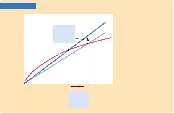
Second, population growth gives us another explanation for why some countries are rich and others are poor. Consider the effects of an increase in population growth. Figure 7-12 shows that an increase in the rate of population
FIGURE 7-12
Investment,
break-even (d + n2)k investment
1. An increase |
(d + n1)k |
in the rate of |
population |
|
growth ... |
sf(k) |
|
The Impact of Population Growth An increase in the rate of population growth from n1 to n2 shifts the line representing population growth and depreciation upward. The new steady
state k* has a lower level of cap-
2
ital per worker than the initial
steady state k*. Thus, the Solow
1
model predicts that economies with higher rates of population growth will have lower levels of capital per worker and therefore lower incomes.
k* |
k* |
Capital |
2 |
1 |
per worker, k |
|
|
2. ... reduces the steadystate capital stock.
214 | P A R T I I I Growth Theory: The Economy in the Very Long Run
growth from n1 to n2 reduces the steady-state level of capital per worker from k*1 to k*2. Because k* is lower and because y* = f(k*), the level of output per worker y* is also lower. Thus, the Solow model predicts that countries with higher population growth will have lower levels of GDP per person. Notice that a change in the population growth rate, like a change in the saving rate, has a level effect on income per person but does not affect the steady-state growth rate of income per person.
Finally, population growth affects our criterion for determining the Golden Rule (consumption-maximizing) level of capital. To see how this criterion changes, note that consumption per worker is
c = y – i.
Because steady-state output is f(k*) and steady-state investment is (d + n)k*, we can express steady-state consumption as
c* = f (k*) − (d + n)k*.
Using an argument largely the same as before, we conclude that the level of k* that maximizes consumption is the one at which
MPK = d + n,
or equivalently,
MPK – d = n.
In the Golden Rule steady state, the marginal product of capital net of depreciation equals the rate of population growth.
CASE STUDY
Population Growth Around the World
Let’s return now to the question of why standards of living vary so much around the world. The analysis we have just completed suggests that population growth may be one of the answers. According to the Solow model, a nation with a high rate of population growth will have a low steady-state capital stock per worker and thus also a low level of income per worker. In other words, high population growth tends to impoverish a country because it is hard to maintain a high level of capital per worker when the number of workers is growing quickly. To see whether the evidence supports this conclusion, we again look at cross-country data.
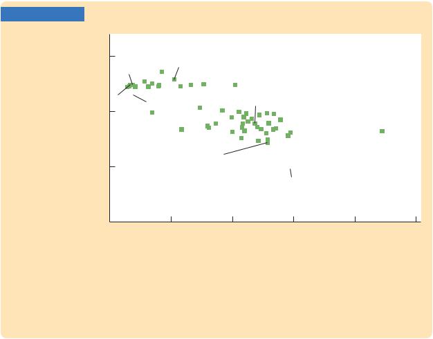
Figure 7-13 is a scatterplot of data for the same 96 countries examined in the previous case study (and in Figure 7-6). The figure shows that countries with high rates of population growth tend to have low levels of income per person. The international evidence is consistent with our model’s prediction that the rate of population growth is one determinant of a country’s standard of living.
This conclusion is not lost on policymakers. Those trying to pull the world’s poorest nations out of poverty, such as the advisers sent to developing
C H A P T E R 7 Economic Growth I: Capital Accumulation and Population Growth | 215
FIGURE 7-13
Income per person
in 2003 (logarithmic scale)
100,000
10,000
1,000
Luxembourg United States
Denmark
Norway |
Canada |
Australia |
Hong Kong |
|
|
|
|
|
|
|
|
|
|
|
|
South Korea |
|
|
Israel |
United |
|
|
|
|
|
|
|
|
|
|
Brazil |
|
|
|
|
|
|
Kingdom Portugal |
|
|
|
|
|
|
|
|
|
|
|
|
|
Uruguay |
Costa Rica |
|
China |
|
|
|
Jamaica |
Guatemala |
Jordan |
India 
Lesotho |
|
|
|
|
|
|
|
|
|
|
|
|
|
|
|
|
|
|
|
|
|
|
|
|
|
|
|
|
|
Cote d’Ivoire |
Pakistan |
|
|
|
|
|
|
|
|
|
|
|
|
|
|
|
|
|
|
|
|
|
|
Gambia |
Burundi |
|
|
|
|
|
|
|
|
|
|
|
|
|
|
|
|
|
|
|
|
|
|
|
|
|
|
|
Guinea-Bissau |
|
|
Ethiopia |
Niger |
100
Population growth (percent per year; average 1960–2003)
International Evidence on Population Growth and Income per Person This figure is a scatterplot of data from 96 countries. It shows that countries with high rates of population growth tend to have low levels of income per person, as the Solow model predicts.
Source: Alan Heston, Robert Summers, and Bettina Aten, Penn World Table Version 6.2, Center for
International Comparisons of Production, Income and Prices at the University of Pennsylvania,
September 2006.
nations by the World Bank, often advocate reducing fertility by increasing education about birth-control methods and expanding women’s job opportunities. Toward the same end, China has followed the totalitarian policy of allowing only one child per couple. These policies to reduce population growth should, if the Solow model is right, raise income per person in the long run.
In interpreting the cross-country data, however, it is important to keep in mind that correlation does not imply causation. The data show that low population growth is typically associated with high levels of income per person, and the Solow model offers one possible explanation for this fact, but other explanations are also possible. It is conceivable that high income encourages low population growth, perhaps because birth-control techniques are more readily available in richer countries. The international data can help us evaluate a theory of growth, such as the Solow model, because they show us whether the theory’s predictions are borne out in the world. But often more than one theory can explain the same facts. ■