
- •About the author
- •Brief Contents
- •Contents
- •Preface
- •This Book’s Approach
- •What’s New in the Seventh Edition?
- •The Arrangement of Topics
- •Part One, Introduction
- •Part Two, Classical Theory: The Economy in the Long Run
- •Part Three, Growth Theory: The Economy in the Very Long Run
- •Part Four, Business Cycle Theory: The Economy in the Short Run
- •Part Five, Macroeconomic Policy Debates
- •Part Six, More on the Microeconomics Behind Macroeconomics
- •Epilogue
- •Alternative Routes Through the Text
- •Learning Tools
- •Case Studies
- •FYI Boxes
- •Graphs
- •Mathematical Notes
- •Chapter Summaries
- •Key Concepts
- •Questions for Review
- •Problems and Applications
- •Chapter Appendices
- •Glossary
- •Translations
- •Acknowledgments
- •Supplements and Media
- •For Instructors
- •Instructor’s Resources
- •Solutions Manual
- •Test Bank
- •PowerPoint Slides
- •For Students
- •Student Guide and Workbook
- •Online Offerings
- •EconPortal, Available Spring 2010
- •eBook
- •WebCT
- •BlackBoard
- •Additional Offerings
- •i-clicker
- •The Wall Street Journal Edition
- •Financial Times Edition
- •Dismal Scientist
- •1-1: What Macroeconomists Study
- •1-2: How Economists Think
- •Theory as Model Building
- •The Use of Multiple Models
- •Prices: Flexible Versus Sticky
- •Microeconomic Thinking and Macroeconomic Models
- •1-3: How This Book Proceeds
- •Income, Expenditure, and the Circular Flow
- •Rules for Computing GDP
- •Real GDP Versus Nominal GDP
- •The GDP Deflator
- •Chain-Weighted Measures of Real GDP
- •The Components of Expenditure
- •Other Measures of Income
- •Seasonal Adjustment
- •The Price of a Basket of Goods
- •The CPI Versus the GDP Deflator
- •The Household Survey
- •The Establishment Survey
- •The Factors of Production
- •The Production Function
- •The Supply of Goods and Services
- •3-2: How Is National Income Distributed to the Factors of Production?
- •Factor Prices
- •The Decisions Facing the Competitive Firm
- •The Firm’s Demand for Factors
- •The Division of National Income
- •The Cobb–Douglas Production Function
- •Consumption
- •Investment
- •Government Purchases
- •Changes in Saving: The Effects of Fiscal Policy
- •Changes in Investment Demand
- •3-5: Conclusion
- •4-1: What Is Money?
- •The Functions of Money
- •The Types of Money
- •The Development of Fiat Money
- •How the Quantity of Money Is Controlled
- •How the Quantity of Money Is Measured
- •4-2: The Quantity Theory of Money
- •Transactions and the Quantity Equation
- •From Transactions to Income
- •The Assumption of Constant Velocity
- •Money, Prices, and Inflation
- •4-4: Inflation and Interest Rates
- •Two Interest Rates: Real and Nominal
- •The Fisher Effect
- •Two Real Interest Rates: Ex Ante and Ex Post
- •The Cost of Holding Money
- •Future Money and Current Prices
- •4-6: The Social Costs of Inflation
- •The Layman’s View and the Classical Response
- •The Costs of Expected Inflation
- •The Costs of Unexpected Inflation
- •One Benefit of Inflation
- •4-7: Hyperinflation
- •The Costs of Hyperinflation
- •The Causes of Hyperinflation
- •4-8: Conclusion: The Classical Dichotomy
- •The Role of Net Exports
- •International Capital Flows and the Trade Balance
- •International Flows of Goods and Capital: An Example
- •Capital Mobility and the World Interest Rate
- •Why Assume a Small Open Economy?
- •The Model
- •How Policies Influence the Trade Balance
- •Evaluating Economic Policy
- •Nominal and Real Exchange Rates
- •The Real Exchange Rate and the Trade Balance
- •The Determinants of the Real Exchange Rate
- •How Policies Influence the Real Exchange Rate
- •The Effects of Trade Policies
- •The Special Case of Purchasing-Power Parity
- •Net Capital Outflow
- •The Model
- •Policies in the Large Open Economy
- •Conclusion
- •Causes of Frictional Unemployment
- •Public Policy and Frictional Unemployment
- •Minimum-Wage Laws
- •Unions and Collective Bargaining
- •Efficiency Wages
- •The Duration of Unemployment
- •Trends in Unemployment
- •Transitions Into and Out of the Labor Force
- •6-5: Labor-Market Experience: Europe
- •The Rise in European Unemployment
- •Unemployment Variation Within Europe
- •The Rise of European Leisure
- •6-6: Conclusion
- •7-1: The Accumulation of Capital
- •The Supply and Demand for Goods
- •Growth in the Capital Stock and the Steady State
- •Approaching the Steady State: A Numerical Example
- •How Saving Affects Growth
- •7-2: The Golden Rule Level of Capital
- •Comparing Steady States
- •The Transition to the Golden Rule Steady State
- •7-3: Population Growth
- •The Steady State With Population Growth
- •The Effects of Population Growth
- •Alternative Perspectives on Population Growth
- •7-4: Conclusion
- •The Efficiency of Labor
- •The Steady State With Technological Progress
- •The Effects of Technological Progress
- •Balanced Growth
- •Convergence
- •Factor Accumulation Versus Production Efficiency
- •8-3: Policies to Promote Growth
- •Evaluating the Rate of Saving
- •Changing the Rate of Saving
- •Allocating the Economy’s Investment
- •Establishing the Right Institutions
- •Encouraging Technological Progress
- •The Basic Model
- •A Two-Sector Model
- •The Microeconomics of Research and Development
- •The Process of Creative Destruction
- •8-5: Conclusion
- •Increases in the Factors of Production
- •Technological Progress
- •The Sources of Growth in the United States
- •The Solow Residual in the Short Run
- •9-1: The Facts About the Business Cycle
- •GDP and Its Components
- •Unemployment and Okun’s Law
- •Leading Economic Indicators
- •9-2: Time Horizons in Macroeconomics
- •How the Short Run and Long Run Differ
- •9-3: Aggregate Demand
- •The Quantity Equation as Aggregate Demand
- •Why the Aggregate Demand Curve Slopes Downward
- •Shifts in the Aggregate Demand Curve
- •9-4: Aggregate Supply
- •The Long Run: The Vertical Aggregate Supply Curve
- •From the Short Run to the Long Run
- •9-5: Stabilization Policy
- •Shocks to Aggregate Demand
- •Shocks to Aggregate Supply
- •10-1: The Goods Market and the IS Curve
- •The Keynesian Cross
- •The Interest Rate, Investment, and the IS Curve
- •How Fiscal Policy Shifts the IS Curve
- •10-2: The Money Market and the LM Curve
- •The Theory of Liquidity Preference
- •Income, Money Demand, and the LM Curve
- •How Monetary Policy Shifts the LM Curve
- •Shocks in the IS–LM Model
- •From the IS–LM Model to the Aggregate Demand Curve
- •The IS–LM Model in the Short Run and Long Run
- •11-3: The Great Depression
- •The Spending Hypothesis: Shocks to the IS Curve
- •The Money Hypothesis: A Shock to the LM Curve
- •Could the Depression Happen Again?
- •11-4: Conclusion
- •12-1: The Mundell–Fleming Model
- •The Goods Market and the IS* Curve
- •The Money Market and the LM* Curve
- •Putting the Pieces Together
- •Fiscal Policy
- •Monetary Policy
- •Trade Policy
- •How a Fixed-Exchange-Rate System Works
- •Fiscal Policy
- •Monetary Policy
- •Trade Policy
- •Policy in the Mundell–Fleming Model: A Summary
- •12-4: Interest Rate Differentials
- •Country Risk and Exchange-Rate Expectations
- •Differentials in the Mundell–Fleming Model
- •Pros and Cons of Different Exchange-Rate Systems
- •The Impossible Trinity
- •12-6: From the Short Run to the Long Run: The Mundell–Fleming Model With a Changing Price Level
- •12-7: A Concluding Reminder
- •Fiscal Policy
- •Monetary Policy
- •A Rule of Thumb
- •The Sticky-Price Model
- •Implications
- •Adaptive Expectations and Inflation Inertia
- •Two Causes of Rising and Falling Inflation
- •Disinflation and the Sacrifice Ratio
- •13-3: Conclusion
- •14-1: Elements of the Model
- •Output: The Demand for Goods and Services
- •The Real Interest Rate: The Fisher Equation
- •Inflation: The Phillips Curve
- •Expected Inflation: Adaptive Expectations
- •The Nominal Interest Rate: The Monetary-Policy Rule
- •14-2: Solving the Model
- •The Long-Run Equilibrium
- •The Dynamic Aggregate Supply Curve
- •The Dynamic Aggregate Demand Curve
- •The Short-Run Equilibrium
- •14-3: Using the Model
- •Long-Run Growth
- •A Shock to Aggregate Supply
- •A Shock to Aggregate Demand
- •A Shift in Monetary Policy
- •The Taylor Principle
- •14-5: Conclusion: Toward DSGE Models
- •15-1: Should Policy Be Active or Passive?
- •Lags in the Implementation and Effects of Policies
- •The Difficult Job of Economic Forecasting
- •Ignorance, Expectations, and the Lucas Critique
- •The Historical Record
- •Distrust of Policymakers and the Political Process
- •The Time Inconsistency of Discretionary Policy
- •Rules for Monetary Policy
- •16-1: The Size of the Government Debt
- •16-2: Problems in Measurement
- •Measurement Problem 1: Inflation
- •Measurement Problem 2: Capital Assets
- •Measurement Problem 3: Uncounted Liabilities
- •Measurement Problem 4: The Business Cycle
- •Summing Up
- •The Basic Logic of Ricardian Equivalence
- •Consumers and Future Taxes
- •Making a Choice
- •16-5: Other Perspectives on Government Debt
- •Balanced Budgets Versus Optimal Fiscal Policy
- •Fiscal Effects on Monetary Policy
- •Debt and the Political Process
- •International Dimensions
- •16-6: Conclusion
- •Keynes’s Conjectures
- •The Early Empirical Successes
- •The Intertemporal Budget Constraint
- •Consumer Preferences
- •Optimization
- •How Changes in Income Affect Consumption
- •Constraints on Borrowing
- •The Hypothesis
- •Implications
- •The Hypothesis
- •Implications
- •The Hypothesis
- •Implications
- •17-7: Conclusion
- •18-1: Business Fixed Investment
- •The Rental Price of Capital
- •The Cost of Capital
- •The Determinants of Investment
- •Taxes and Investment
- •The Stock Market and Tobin’s q
- •Financing Constraints
- •Banking Crises and Credit Crunches
- •18-2: Residential Investment
- •The Stock Equilibrium and the Flow Supply
- •Changes in Housing Demand
- •18-3: Inventory Investment
- •Reasons for Holding Inventories
- •18-4: Conclusion
- •19-1: Money Supply
- •100-Percent-Reserve Banking
- •Fractional-Reserve Banking
- •A Model of the Money Supply
- •The Three Instruments of Monetary Policy
- •Bank Capital, Leverage, and Capital Requirements
- •19-2: Money Demand
- •Portfolio Theories of Money Demand
- •Transactions Theories of Money Demand
- •The Baumol–Tobin Model of Cash Management
- •19-3 Conclusion
- •Lesson 2: In the short run, aggregate demand influences the amount of goods and services that a country produces.
- •Question 1: How should policymakers try to promote growth in the economy’s natural level of output?
- •Question 2: Should policymakers try to stabilize the economy?
- •Question 3: How costly is inflation, and how costly is reducing inflation?
- •Question 4: How big a problem are government budget deficits?
- •Conclusion
- •Glossary
- •Index

C H A P T E R 5 The Open Economy | 135
resented by the variable A). For example, compared to rich nations, poor nations may have less access to advanced technologies, lower levels of education (or human capital ), or less efficient economic policies. Such differences could mean less output for given inputs of capital and labor; in the Cobb–Douglas production function, this is translated into a lower value of the parameter A. If so, then capital need not be more valuable in poor nations, even though capital is scarce.
A second reason capital might not flow to poor nations is that property rights are often not enforced. Corruption is much more prevalent; revolutions, coups, and expropriation of wealth are more common; and governments often default on their debts. So even if capital is more valuable in poor nations, foreigners may avoid investing their wealth there simply because they are afraid of losing it. Moreover, local investors face similar incentives. Imagine that you live in a poor nation and are lucky enough to have some wealth to invest; you might well decide that putting it in a safe country like the United States is your best option, even if capital is less valuable there than in your home country.
Whichever of these two reasons is correct, the challenge for poor nations is to find ways to reverse the situation. If these nations offered the same production efficiency and legal protections as the U.S. economy, the direction of international capital flows would likely reverse. The U.S. trade deficit would become a trade surplus, and capital would flow to these emerging nations. Such a change would help the poor of the world escape poverty.2 ■
5-3 Exchange Rates
Having examined the international flows of capital and of goods and services, we now extend the analysis by considering the prices that apply to these transactions. The exchange rate between two countries is the price at which residents of those countries trade with each other. In this section we first examine precisely what the exchange rate measures, and we then discuss how exchange rates are determined.
Nominal and Real Exchange Rates
Economists distinguish between two exchange rates: the nominal exchange rate and the real exchange rate. Let’s discuss each in turn and see how they are related.
The Nominal Exchange Rate The nominal exchange rate is the relative price of the currencies of two countries. For example, if the exchange rate between the U.S. dollar and the Japanese yen is 120 yen per dollar, then you can
2 For more on this topic, see Robert E. Lucas, “Why Doesn’t Capital Flow from Rich to Poor Countries?” American Economic Review 80 (May 1990): 92–96.
136 | P A R T I I Classical Theory: The Economy in the Long Run
exchange one dollar for 120 yen in world markets for foreign currency. A Japanese who wants to obtain dollars would pay 120 yen for each dollar he bought. An American who wants to obtain yen would get 120 yen for each dollar he paid. When people refer to “the exchange rate’’ between two countries, they usually mean the nominal exchange rate.
Notice that an exchange rate can be reported in two ways. If one dollar buys 120 yen, then one yen buys 0.00833 dollar. We can say the exchange rate is 120 yen per dollar, or we can say the exchange rate is 0.00833 dollar per yen. Because 0.00833 equals 1/120, these two ways of expressing the exchange rate are equivalent.
This book always expresses the exchange rate in units of foreign currency per dollar. With this convention, a rise in the exchange rate—say, from 120 to 125 yen per dollar—is called an appreciation of the dollar; a fall in the exchange rate is called a depreciation. When the domestic currency appreciates, it buys more of the foreign currency; when it depreciates, it buys less. An appreciation is sometimes called a strengthening of the currency, and a depreciation is sometimes called a weakening of the currency.
The Real Exchange Rate The real exchange rate is the relative price of the goods of two countries. That is, the real exchange rate tells us the rate at which we can trade the goods of one country for the goods of another. The real exchange rate is sometimes called the terms of trade.
To see the relation between the real and nominal exchange rates, consider a single good produced in many countries: cars. Suppose an American car costs $10,000 and a similar Japanese car costs 2,400,000 yen. To compare the prices of the two cars, we must convert them into a common currency. If a dollar is worth 120 yen, then the American car costs 1,200,000 yen. Comparing the price of the American car (1,200,000 yen) and the price of the Japanese car (2,400,000 yen), we conclude that the American car costs one-half of what the Japanese car costs. In other words, at current prices, we can exchange 2 American cars for 1 Japanese car.
We can summarize our calculation as follows:
Real Exchange |
= |
(120 yen/dollar) × (10,000 dollars/American Car) |
||
Rate |
|
|||
|
|
(2,400,000 yen/Japanese Car) |
||
|
= 0.5 |
Japanese Car |
. |
|
|
|
|||
|
|
|
American Car |
At these prices and this exchange rate, we obtain one-half of a Japanese car per American car. More generally, we can write this calculation as
Real Exchange = |
Nominal Exchange Rate × Price of Domestic Good |
. |
|
||
Rate |
Price of Foreign Good |
The rate at which we exchange foreign and domestic goods depends on the prices of the goods in the local currencies and on the rate at which the currencies are exchanged.

C H A P T E R 5 The Open Economy | 137
This calculation of the real exchange rate for a single good suggests how we should define the real exchange rate for a broader basket of goods. Let e be the nominal exchange rate (the number of yen per dollar), P be the price level in the United States (measured in dollars), and P * be the price level in Japan (measured
in yen). Then the real exchange rate e is |
|
||
Real |
|
Nominal |
Ratio of |
Exchange = Exchange × Price |
|||
Rate |
|
Rate |
Levels |
e |
= |
e |
× (P/P *). |
The real exchange rate between two countries is computed from the nominal exchange rate and the price levels in the two countries. If the real exchange rate is high, foreign goods are relatively cheap, and domestic goods are relatively expensive. If the real exchange rate is low, foreign goods are relatively expensive, and domestic goods are relatively cheap.
The Real Exchange Rate and the Trade Balance
What macroeconomic influence does the real exchange rate exert? To answer this question, remember that the real exchange rate is nothing more than a relative price. Just as the relative price of hamburgers and pizza determines which you choose for lunch, the relative price of domestic and
foreign goods affects the demand for these goods. Suppose first that the real exchange rate is low. In
this case, because domestic goods are relatively cheap, domestic residents will want to purchase fewer imported goods: they will buy Fords rather than Toyotas, drink Coors rather than Heineken, and vacation in Florida rather than Italy. For the same reason, foreigners will want to buy many of our goods. As a result of both of these actions, the quantity of our net exports demanded will be high.
The opposite occurs if the real exchange rate is high. Because domestic goods are expensive relative to foreign goods, domestic residents will want to buy many imported goods, and foreigners will want to buy few of our goods. Therefore, the quantity of our net exports demanded will be low.
We write this relationship between the real exchange rate and net exports as
NX = NX(e).
This equation states that net exports are a function of the real exchange rate. Figure 5-7 illustrates the negative relationship between the trade balance and the real exchange rate.
by Matteson; © 1988 |
Yorker Magazine, Inc. |
Drawing |
The New |

138 | P A R T I I Classical Theory: The Economy in the Long Run
FIGURE 5-7
Real exchange rate, e
NX(e)
0 |
Net exports, NX |
Net Exports and the Real Exchange Rate The figure shows the relationship between the real exchange rate and net exports: the lower the real exchange rate, the less expensive are domestic goods relative to foreign goods, and thus the greater are our net exports. Note that
a portion of the horizontal axis measures negative values of NX: because imports can exceed exports, net exports can be less than zero.
The Determinants of the Real Exchange Rate
We now have all the pieces needed to construct a model that explains what factors determine the real exchange rate. In particular, we combine the relationship between net exports and the real exchange rate we just discussed with the model of the trade balance we developed earlier in the chapter. We can summarize the analysis as follows:
■The real exchange rate is related to net exports. When the real exchange rate is lower, domestic goods are less expensive relative to foreign goods, and net exports are greater.
■The trade balance (net exports) must equal the net capital outflow, which in turn equals saving minus investment. Saving is fixed by the consumption function and fiscal policy; investment is fixed by the investment function and the world interest rate.
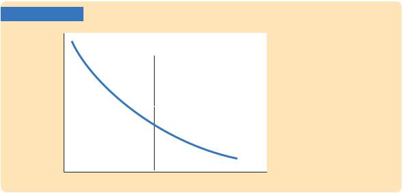
Figure 5-8 illustrates these two conditions. The line showing the relationship between net exports and the real exchange rate slopes downward because a low real exchange rate makes domestic goods relatively inexpensive. The line representing the excess of saving over investment, S − I, is vertical because neither saving nor investment depends on the real exchange rate. The crossing of these two lines determines the equilibrium real exchange rate.
Figure 5-8 looks like an ordinary supply-and-demand diagram. In fact, you can think of this diagram as representing the supply and demand for foreign-currency exchange. The vertical line, S − I, represents the net capital outflow and thus the supply of dollars to be exchanged into foreign currency and invested abroad. The downward-sloping line, NX(e), represents the net demand for dollars coming from