

54 | P A R T I I Classical Theory: The Economy in the Long Run
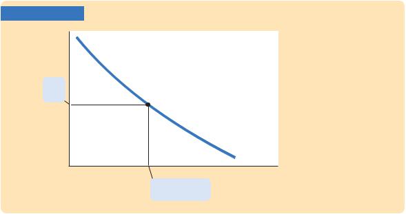
FIGURE 3-4
Units of output
Real wage
The Marginal Product of Labor Schedule The marginal product of labor MPL depends on the amount of labor. The MPL curve slopes downward because the MPL declines as L increases. The firm hires labor up to the point where the real wage W/P equals the MPL. Hence, this schedule is also the firm’s labor demand curve.
MPL, Labor demand
Units of labor, L
Quantity of labor demanded
Like labor, capital is subject to diminishing marginal product. Once again consider the production of bread at a bakery. The first several ovens installed in the kitchen will be very productive. However, if the bakery installs more and more ovens, while holding its labor force constant, it will eventually contain more ovens than its employees can effectively operate. Hence, the marginal product of the last few ovens is lower than that of the first few.
The increase in profit from renting an additional machine is the extra revenue from selling the output of that machine minus the machine’s rental price:
Profit = Revenue − Cost
= (P × MPK ) − R.
To maximize profit, the firm continues to rent more capital until the MPK falls to equal the real rental price:
MPK = R/P.
The real rental price of capital is the rental price measured in units of goods rather than in dollars.
To sum up, the competitive, profit-maximizing firm follows a simple rule about how much labor to hire and how much capital to rent. The firm demands each factor of production until that factor’s marginal product falls to equal its real factor price.
The Division of National Income
Having analyzed how a firm decides how much of each factor to employ, we can now explain how the markets for the factors of production distribute the economy’s total income. If all firms in the economy are competitive and profit

C H A P T E R 3 National Income: Where It Comes From and Where It Goes | 55
maximizing, then each factor of production is paid its marginal contribution to the production process. The real wage paid to each worker equals the MPL, and the real rental price paid to each owner of capital equals the MPK. The total real wages paid to labor are therefore MPL × L, and the total real return paid to capital owners is MPK × K.
The income that remains after the firms have paid the factors of production is the economic profit of the owners of the firms. Real economic profit is
Economic Profit =Y − (MPL × L) − (MPK × K ).
Because we want to examine the distribution of national income, we rearrange the terms as follows:
Y = (MPL × L) + (MPK × K ) + Economic Profit.
Total income is divided among the return to labor, the return to capital, and economic profit.
How large is economic profit? The answer is surprising: if the production function has the property of constant returns to scale, as is often thought to be the case, then economic profit must be zero. That is, nothing is left after the factors of production are paid. This conclusion follows from a famous mathematical result called Euler’s theorem,2 which states that if the production function has constant returns to scale, then
F(K, L) = (MPK × K) + (MPL × L).
If each factor of production is paid its marginal product, then the sum of these factor payments equals total output. In other words, constant returns to scale, profit maximization, and competition together imply that economic profit is zero.
If economic profit is zero, how can we explain the existence of “profit” in the economy? The answer is that the term “profit” as normally used is different from economic profit. We have been assuming that there are three types of agents: workers, owners of capital, and owners of firms. Total income is divided among wages, return to capital, and economic profit. In the real world, however, most firms own rather than rent the capital they use. Because firm owners and capital owners are the same people, economic profit and the return to capital are often lumped together. If we call this alternative definition accounting profit, we can say that
Accounting Profit = Economic Profit + (MPK × K ).
2 Mathematical note: To prove Euler’s theorem, we need to use some multivariate calculus. Begin with the definition of constant returns to scale: zY = F(zK, zL). Now differentiate with respect to z to obtain:
Y = F1(zK, zL) K + F2(zK, zL) L,
where F1 and F2 denote partial derivatives with respect to the first and second arguments of the function. Evaluating this expression at z = 1, and noting that the partial derivatives equal the marginal products, yields Euler’s theorem.

56 | P A R T I I Classical Theory: The Economy in the Long Run
Under our assumptions—constant returns to scale, profit maximization, and competition—economic profit is zero. If these assumptions approximately describe the world, then the “profit” in the national income accounts must be mostly the return to capital.
We can now answer the question posed at the beginning of this chapter about how the income of the economy is distributed from firms to households. Each factor of production is paid its marginal product, and these factor payments exhaust total output. Total output is divided between the payments to capital and the payments to labor, depending on their marginal productivities.
CASE STUDY
The Black Death and Factor Prices
According to the neoclassical theory of distribution, factor prices equal the marginal products of the factors of production. Because the marginal products depend on the quantities of the factors, a change in the quantity of any one factor alters the marginal products of all the factors. Therefore, a change in the supply of a factor alters equilibrium factor prices and the distribution of income.
Fourteenth-century Europe provides a grisly natural experiment to study how factor quantities affect factor prices. The outbreak of the bubonic plague—the Black Death—in 1348 reduced the population of Europe by about one-third within a few years. Because the marginal product of labor increases as the amount of labor falls, this massive reduction in the labor force should have raised the marginal product of labor and equilibrium real wages. (That is, the economy should have moved to the left along the curves in Figures 3-3 and 3-4.) The evidence confirms the theory: real wages approximately doubled during the plague years. The peasants who were fortunate enough to survive the plague enjoyed economic prosperity.
The reduction in the labor force caused by the plague should also have affected the return to land, the other major factor of production in medieval Europe. With fewer workers available to farm the land, an additional unit of land would have produced less additional output, and so land rents should have fallen. Once again, the theory is confirmed: real rents fell 50 percent or more during this period. While the peasant classes prospered, the landed classes suffered reduced incomes.3 ■
The Cobb–Douglas Production Function
What production function describes how actual economies turn capital and labor into GDP? One answer to this question came from a historic collaboration between a U.S. senator and a mathematician.
3 Carlo M. Cipolla, Before the Industrial Revolution: European Society and Economy, 1000 –1700,
2nd ed. (New York: Norton, 1980), 200–202.

C H A P T E R 3 National Income: Where It Comes From and Where It Goes | 57
Paul Douglas was a U.S. senator from Illinois from 1949 to 1966. In 1927, however, when he was still a professor of economics, he noticed a surprising fact: the division of national income between capital and labor had been roughly constant over a long period. In other words, as the economy grew more prosperous over time, the total income of workers and the total income of capital owners grew at almost exactly the same rate. This observation caused Douglas to wonder what conditions might lead to constant factor shares.
Douglas asked Charles Cobb, a mathematician, what production function, if any, would produce constant factor shares if factors always earned their marginal products. The production function would need to have the property that
Capital Income = MPK × K = Y
and
Labor Income = MPL × L = (1 – ) Y,
where is a constant between zero and one that measures capital’s share of income. That is, determines what share of income goes to capital and what share goes to labor. Cobb showed that the function with this property is
F(K, L) = A K L1− ,
where A is a parameter greater than zero that measures the productivity of the available technology. This function became known as the Cobb–Douglas production function.
Let’s take a closer look at some of the properties of this production function. First, the Cobb–Douglas production function has constant returns to scale. That is, if capital and labor are increased by the same proportion, then output increases by that proportion as well.4
4 Mathematical note: To prove that the Cobb–Douglas production function has constant returns to scale, examine what happens when we multiply capital and labor by a constant z:
F(zK, zL) = A(zK) (z L)1− .
Expanding terms on the right,
F(zK, zL) = Az K z1− L1− .
Rearranging to bring like terms together, we get
F(zK, zL) = Az z1− K L1− .
Since z z1− = z, our function becomes
F(zK, zL) = z A K L1− .
But A K L1− = F(K, L). Thus,
F(zK, zL) = zF(K, L) = zY.
Hence, the amount of output Y increases by the same factor z, which implies that this production function has constant returns to scale.

58 | P A R T I I Classical Theory: The Economy in the Long Run
Next, consider the marginal products for the Cobb–Douglas production function. The marginal product of labor is5
MPL = (1 − ) A K L− ,
and the marginal product of capital is
MPK = A K α −1L1−α.
From these equations, recalling that is between zero and one, we can see what causes the marginal products of the two factors to change. An increase in the amount of capital raises the MPL and reduces the MPK. Similarly, an increase in the amount of labor reduces the MPL and raises the MPK. A technological advance that increases the parameter A raises the marginal product of both factors proportionately.
The marginal products for the Cobb–Douglas production function can also be written as6
MPL = (1 − )Y/L.
MPK = Y/K.
The MPL is proportional to output per worker, and the MPK is proportional to output per unit of capital. Y/L is called average labor productivity, and Y/K is called average capital productivity. If the production function is Cobb–Douglas, then the marginal productivity of a factor is proportional to its average productivity.
We can now verify that if factors earn their marginal products, then the parameter indeed tells us how much income goes to labor and how much goes to capital. The total amount paid to labor, which we have seen is MPL × L, equals (1 − )Y. Therefore, (1 − ) is labor’s share of output. Similarly, the total amount paid to capital, MPK × K, equals Y, and is capital’s share of output. The ratio of labor income to capital income is a constant, (1 − )/ , just as Douglas observed. The factor shares depend only on the parameter , not on the amounts of capital or labor or on the state of technology as measured by the parameter A.
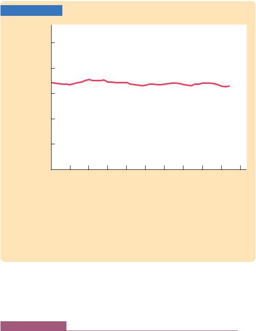
More recent U.S. data are also consistent with the Cobb–Douglas production function. Figure 3-5 shows the ratio of labor income to total income in the United States from 1960 to 2007. Despite the many changes in the economy over the past four decades, this ratio has remained about 0.7. This division of income is easily explained by a Cobb–Douglas production function in which the parameter is about 0.3. According to this parameter, capital receives 30 percent of income, and labor receives 70 percent.
5 Mathematical note: Obtaining the formulas for the marginal products from the production function requires a bit of calculus. To find the MPL, differentiate the production function with respect to L. This is done by multiplying by the exponent (1 − ) and then subtracting 1 from the old exponent to obtain the new exponent, − . Similarly, to obtain the MPK, differentiate the production function with respect to K.
6 Mathematical note: To check these expressions for the marginal products, substitute in the production function for Y to show that these expressions are equivalent to the earlier formulas for the marginal products.
C H A P T E R 3 National Income: Where It Comes From and Where It Goes | 59
FIGURE 3-5 |
|
|
|
|
|
|
|
|
|
|
Labor’s share |
|
|
|
|
|
|
|
|
|
|
of total income |
|
|
|
|
|
|
|
|
|
|
1.0 |
|
|
|
|
|
|
|
|
|
|
0.8 |
|
|
|
|
|
|
|
|
|
|
0.6 |
|
|
|
|
|
|
|
|
|
|
0.4 |
|
|
|
|
|
|
|
|
|
|
0.2 |
|
|
|
|
|
|
|
|
|
|
0 |
1965 |
1970 |
1975 |
1980 |
1985 |
1990 |
1995 |
2000 |
2005 |
2010 |
1960 |
||||||||||
|
|
|
|
|
|
|
|
|
|
Year |
The Ratio of Labor Income to Total Income Labor income has remained about 0.7 of total income over a long period of time. This approximate constancy of factor shares is consistent with the Cobb–Douglas production function.
Source: U.S. Department of Commerce. This figure is produced from U.S. national income accounts data. Labor income is compensation of employees. Total income is the sum of labor income, corporate profits, net interest, rental income, and depreciation. Proprietors’ income is excluded from these calculations, because it is a combination of labor income and capital income.
The Cobb–Douglas production function is not the last word in explaining the economy’s production of goods and services or the distribution of national income between capital and labor. It is, however, a good place to start.
CASE STUDY
Labor Productivity as the Key Determinant
of Real Wages
The neoclassical theory of distribution tells us that the real wage W/P equals the marginal product of labor. The Cobb–Douglas production function tells us that the marginal product of labor is proportional to average labor productivity Y/L. If this theory is right, then workers should enjoy rapidly rising living standards when labor productivity is growing robustly. Is this true?
Table 3-1 presents some data on growth in productivity and real wages for the U.S. economy. From 1959 to 2007, productivity as measured by output per hour

60 | P A R T I I Classical Theory: The Economy in the Long Run
TA B L E 3-1
Growth in Labor Productivity and Real Wages: The U.S. Experience
|
Growth Rate |
Growth Rate |
Time Period |
of Labor Productivity |
of Real Wages |
|
|
|
1959–2007 |
2.1% |
2.0% |
1959–1973 |
2.8 |
2.8 |
1973–1995 |
1.4 |
1.2 |
1995–2007 |
2.5 |
2.4 |
Source: Economic Report of the President 2008, Table B-49, and updates from the U.S. Department of Commerce website. Growth in labor productivity is measured here as the annualized rate of change in output per hour in the nonfarm business sector. Growth in real wages is measured as the annualized change in compensation per hour in the nonfarm business sector divided by the implicit price deflator for that sector.
of work grew about 2.1 percent per year. Real wages grew at 2.0 percent—almost exactly the same rate. With a growth rate of 2 percent per year, productivity and real wages double about every 35 years.
Productivity growth varies over time. The table shows the data for three shorter periods that economists have identified as having different productivity experiences. (A case study in Chapter 8 examines the reasons for these changes in productivity growth.) Around 1973, the U.S. economy experienced a significant slowdown in productivity growth that lasted until 1995. The cause of the productivity slowdown is not well understood, but the link between productivity and real wages was exactly as standard theory predicts. The slowdown in productivity growth from 2.8 to 1.4 percent per year coincided with a slowdown in real wage growth from 2.8 to 1.2 percent per year.
Productivity growth picked up again around 1995, and many observers hailed the arrival of the “new economy.” This productivity acceleration is often attributed to the spread of computers and information technology. As theory predicts, growth in real wages picked up as well. From 1995 to 2007, productivity grew by 2.5 percent per year and real wages by 2.4 percent per year.
Theory and history both confirm the close link between labor productivity and real wages. This lesson is the key to understanding why workers today are better off than workers in previous generations. ■
3-3 What Determines the Demand
for Goods and Services?
We have seen what determines the level of production and how the income from production is distributed to workers and owners of capital. We now continue our tour of the circular flow diagram, Figure 3-1, and examine how the output from production is used.