

20 | P A R T I Introduction
Stocks and Flows
|
Many |
economic variables measure a quantity of |
||
|
something—a quantity of money, a quantity of |
|||
|
goods, and so on. Economists distinguish between |
|||
|
two types of quantity variables: stocks and flows. A |
|||
|
stock is a quantity measured at a given point in |
|||
|
time, whereas a flow is a quantity measured per |
|||
|
unit of time. |
|
||
|
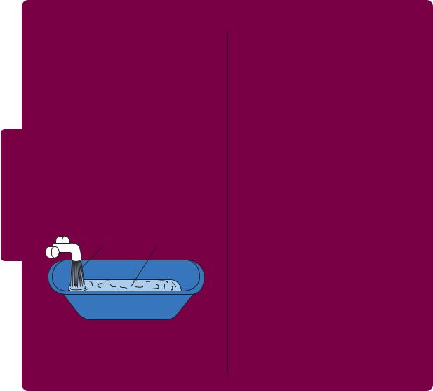
A bathtub, shown in Figure 2-2, is the classic |
|||
|
example used to illustrate stocks and flows. The |
|||
|
amount of water in the tub is a stock: it is the |
|||
|
quantity of water in the tub at a given point in |
|||
|
time. The amount of water coming out of the |
|||
FYI |
faucet is a flow: it is the quantity of water being |
|||
added to the tub per unit of time. Note that we |
||||
|
||||
|
measure stocks and flows in different units. We |
|||
|
say that the bathtub contains 50 gallons of water, |
|||
|
|
Flow |
Stock |
|
Figure 2-2 Stocks and Flows The amount of water in a bathtub is a stock: it is a quantity measured at a given moment in time. The amount of water coming out of the faucet is a flow: it is a quantity measured per unit of time.
but that water is coming out of the faucet at 5 gallons per minute.
GDP is probably the most important flow variable in economics: it tells us how many dollars are flowing around the economy’s circular flow per unit of time. When you hear someone say that the U.S. GDP is $14 trillion, you should understand that this means that it is $14 trillion per year. (Equivalently, we could say that U.S. GDP is $444,000 per second.)
Stocks and flows are often related. In the bathtub example, these relationships are clear. The stock of water in the tub represents the accumulation of the flow out of the faucet, and the flow of water represents the change in the stock. When building theories to explain economic variables, it is often useful to determine whether the variables are stocks or flows and whether any relationships link them.
Here are some examples of related stocks and flows that we study in future chapters:
A person’s wealth is a stock; his income and expenditure are flows.
The number of unemployed people is a stock; the number of people losing their jobs is a flow.
The amount of capital in the economy is a stock; the amount of investment is a flow.
The government debt is a stock; the government budget deficit is a flow.
on total income. If the firm produces the extra loaf without hiring any more labor (such as by making the production process more efficient), then profit increases. If the firm produces the extra loaf by hiring more labor, then wages increase. In both cases, expenditure and income increase equally.
Rules for Computing GDP
In an economy that produces only bread, we can compute GDP by adding up the total expenditure on bread. Real economies, however, include the production and sale of a vast number of goods and services. To compute GDP for such a complex economy, it will be helpful to have a more precise definition:
C H A P T E R 2 The Data of Macroeconomics | 21
Gross domestic product (GDP) is the market value of all final goods and services produced within an economy in a given period of time. To see how this definition is applied, let’s discuss some of the rules that economists follow in constructing this statistic.
Adding Apples and Oranges The U.S. economy produces many different goods and services—hamburgers, haircuts, cars, computers, and so on. GDP combines the value of these goods and services into a single measure. The diversity of products in the economy complicates the calculation of GDP because different products have different values.
Suppose, for example, that the economy produces four apples and three oranges. How do we compute GDP? We could simply add apples and oranges and conclude that GDP equals seven pieces of fruit. But this makes sense only if we thought apples and oranges had equal value, which is generally not true. (This would be even clearer if the economy had produced four watermelons and three grapes.)
To compute the total value of different goods and services, the national income accounts use market prices because these prices reflect how much people are willing to pay for a good or service. Thus, if apples cost $0.50 each and oranges cost $1.00 each, GDP would be
GDP = (Price of Apples × Quantity of Apples)
+ (Price of Oranges × Quantity of Oranges)
=($0.50 × 4) + ($1.00 × 3)
=$5.00.
GDP equals $5.00—the value of all the apples, $2.00, plus the value of all the oranges, $3.00.
Used Goods When the Topps Company makes a package of baseball cards and sells it for 50 cents, that 50 cents is added to the nation’s GDP. But what about when a collector sells a rare Mickey Mantle card to another collector for $500? That $500 is not part of GDP. GDP measures the value of currently produced goods and services. The sale of the Mickey Mantle card reflects the transfer of an asset, not an addition to the economy’s income. Thus, the sale of used goods is not included as part of GDP.
The Treatment of Inventories Imagine that a bakery hires workers to produce more bread, pays their wages, and then fails to sell the additional bread. How does this transaction affect GDP?
The answer depends on what happens to the unsold bread. Let’s first suppose that the bread spoils. In this case, the firm has paid more in wages but has not received any additional revenue, so the firm’s profit is reduced by the amount that wages have increased. Total expenditure in the economy hasn’t changed because no one buys the bread. Total income hasn’t changed either—although more is distributed as wages and less as profit. Because the transaction affects neither expenditure nor income, it does not alter GDP.
22 | P A R T I Introduction
Now suppose, instead, that the bread is put into inventory to be sold later. In this case, the transaction is treated differently. The owners of the firm are assumed to have “purchased’’ the bread for the firm’s inventory, and the firm’s profit is not reduced by the additional wages it has paid. Because the higher wages raise total income, and greater spending on inventory raises total expenditure, the economy’s GDP rises.
What happens later when the firm sells the bread out of inventory? This case is much like the sale of a used good. There is spending by bread consumers, but there is inventory disinvestment by the firm. This negative spending by the firm offsets the positive spending by consumers, so the sale out of inventory does not affect GDP.
The general rule is that when a firm increases its inventory of goods, this investment in inventory is counted as an expenditure by the firm owners. Thus, production for inventory increases GDP just as much as production for final sale. A sale out of inventory, however, is a combination of positive spending (the purchase) and negative spending (inventory disinvestment), so it does not influence GDP. This treatment of inventories ensures that GDP reflects the economy’s current production of goods and services.
Intermediate Goods and Value Added Many goods are produced in stages: raw materials are processed into intermediate goods by one firm and then sold to another firm for final processing. How should we treat such products when computing GDP? For example, suppose a cattle rancher sells one-quarter pound of meat to McDonald’s for $0.50, and then McDonald’s sells you a hamburger for $1.50. Should GDP include both the meat and the hamburger (a total of $2.00), or just the hamburger ($1.50)?
The answer is that GDP includes only the value of final goods. Thus, the hamburger is included in GDP but the meat is not: GDP increases by $1.50, not by $2.00. The reason is that the value of intermediate goods is already included as part of the market price of the final goods in which they are used. To add the intermediate goods to the final goods would be double counting—that is, the meat would be counted twice. Hence, GDP is the total value of final goods and services produced.
One way to compute the value of all final goods and services is to sum the value added at each stage of production. The value added of a firm equals the value of the firm’s output less the value of the intermediate goods that the firm purchases. In the case of the hamburger, the value added of the rancher is $0.50 (assuming that the rancher bought no intermediate goods), and the value added of McDonald’s is $1.50 – $0.50, or $1.00. Total value added is $0.50 + $1.00, which equals $1.50. For the economy as a whole, the sum of all value added must equal the value of all final goods and services. Hence, GDP is also the total value added of all firms in the economy.
Housing Services and Other Imputations Although most goods and services are valued at their market prices when computing GDP, some are not sold in the marketplace and therefore do not have market prices. If GDP is to include the value of these goods and services, we must use an estimate of their value. Such an estimate is called an imputed value.
C H A P T E R 2 The Data of Macroeconomics | 23
Imputations are especially important for determining the value of housing. A person who rents a house is buying housing services and providing income for the landlord; the rent is part of GDP, both as expenditure by the renter and as income for the landlord. Many people, however, live in their own homes. Although they do not pay rent to a landlord, they are enjoying housing services similar to those that renters purchase. To take account of the housing services enjoyed by homeowners, GDP includes the “rent” that these homeowners “pay” to themselves. Of course, homeowners do not in fact pay themselves this rent. The Department of Commerce estimates what the market rent for a house would be if it were rented and includes that imputed rent as part of GDP. This imputed rent is included both in the homeowner’s expenditure and in the homeowner’s income.
Imputations also arise in valuing government services. For example, police officers, firefighters, and senators provide services to the public. Giving a value to these services is difficult because they are not sold in a marketplace and therefore do not have a market price. The national income accounts include these services in GDP by valuing them at their cost. That is, the wages of these public servants are used as a measure of the value of their output.
In many cases, an imputation is called for in principle but, to keep things simple, is not made in practice. Because GDP includes the imputed rent on owner-occupied houses, one might expect it also to include the imputed rent on cars, lawn mowers, jewelry, and other durable goods owned by households. Yet the value of these rental services is left out of GDP. In addition, some of the output of the economy is produced and consumed at home and never enters the marketplace. For example, meals cooked at home are similar to meals cooked at a restaurant, yet the value added in meals at home is left out of GDP.
Finally, no imputation is made for the value of goods and services sold in the underground economy. The underground economy is the part of the economy that people hide from the government either because they wish to evade taxation or because the activity is illegal. Examples include domestic workers paid “off the books” and the illegal drug trade.
Because the imputations necessary for computing GDP are only approximate, and because the value of many goods and services is left out altogether, GDP is an imperfect measure of economic activity. These imperfections are most problematic when comparing standards of living across countries. The size of the underground economy, for instance, varies widely from country to country. Yet as long as the magnitude of these imperfections remains fairly constant over time, GDP is useful for comparing economic activity from year to year.
Real GDP Versus Nominal GDP
Economists use the rules just described to compute GDP, which values the economy’s total output of goods and services. But is GDP a good measure of economic well-being? Consider once again the economy that produces only apples
24 | P A R T I Introduction
and oranges. In this economy GDP is the sum of the value of all the apples produced and the value of all the oranges produced. That is,
GDP = (Price of Apples × Quantity of Apples)
+ (Price of Oranges × Quantity of Oranges).
Economists call the value of goods and services measured at current prices nominal GDP. Notice that nominal GDP can increase either because prices rise or because quantities rise.
It is easy to see that GDP computed this way is not a good gauge of economic well-being. That is, this measure does not accurately reflect how well the economy can satisfy the demands of households, firms, and the government. If all prices doubled without any change in quantities, nominal GDP would double. Yet it would be misleading to say that the economy’s ability to satisfy demands has doubled, because the quantity of every good produced remains the same.
A better measure of economic well-being would tally the economy’s output of goods and services without being influenced by changes in prices. For this purpose, economists use real GDP, which is the value of goods and services measured using a constant set of prices. That is, real GDP shows what would have happened to expenditure on output if quantities had changed but prices had not.
To see how real GDP is computed, imagine we wanted to compare output in 2009 with output in subsequent years for our apple-and-orange economy. We could begin by choosing a set of prices, called base-year prices, such as the prices that prevailed in 2009. Goods and services are then added up using these base-year prices to value the different goods in each year. Real GDP for 2009 would be
Real GDP = (2009 Price of Apples × 2009 Quantity of Apples)
+ (2009 Price of Oranges × 2009 Quantity of Oranges).
Similarly, real GDP in 2010 would be
Real GDP = (2009 Price of Apples × 2010 Quantity of Apples)
+ (2009 Price of Oranges × 2010 Quantity of Oranges).
And real GDP in 2011 would be
Real GDP = (2009 Price of Apples × 2011 Quantity of Apples)
+ (2009 Price of Oranges × 2011 Quantity of Oranges).
Notice that 2009 prices are used to compute real GDP for all three years. Because the prices are held constant, real GDP varies from year to year only if the quantities produced vary. Because a society’s ability to provide economic satisfaction for its members ultimately depends on the quantities of goods and services produced, real GDP provides a better measure of economic well-being than nominal GDP.