

Working with R |
11 |
|
Table 1.2 R help functions |
|
|
|
|
|
Function |
Action |
|
|
|
|
help.start() |
General help |
|
help("foo") or ?foo |
Help on function foo (quotation marks optional) |
|
help.search("foo") or ??foo |
Searches the help system for instances of the string |
|
|
foo |
|
example("foo") |
Examples of function foo (quotation marks optional) |
|
RSiteSearch("foo") |
Searches for the string foo in online help manuals and |
|
|
archived mailing lists |
|
apropos("foo", mode="function") |
Lists all available functions with foo in their name |
|
data() |
Lists all available example datasets contained in cur- |
|
|
rently loaded packages |
|
vignette() |
Lists all available vignettes for currently installed pack- |
|
|
ages |
|
vignette("foo") |
Displays specific vignettes for topic foo |
|
|
|
|
The function help.start() opens a browser window with access to introductory and advanced manuals, FAQs, and reference materials. The RSiteSearch() function searches for a given topic in online help manuals and archives of the R-Help discussion list and returns the results in a browser window. The vignettes returned by the vignette() function are practical introductory articles provided in PDF format. Not all packages have vignettes.
As you can see, R provides extensive help facilities, and learning to navigate them will definitely aid your programming efforts. It’s a rare session that I don’t use ? to look up the features (such as options or return values) of some function.
1.3.3The workspace
The workspace is your current R working environment and includes any user-defined objects (vectors, matrices, functions, data frames, and lists). At the end of an R session, you can save an image of the current workspace that’s automatically reloaded the next time R starts. Commands are entered interactively at the R user prompt. You can use the up and down arrow keys to scroll through your command history. Doing so allows you to select a previous command, edit it if desired, and resubmit it using the Enter key.
The current working directory is the directory from which R will read files and to which it will save results by default. You can find out what the current working directory is by using the getwd() function. You can set the current working directory by using the setwd() function. If you need to input a file that isn’t in the current working directory, use the full pathname in the call. Always enclose the names of files and
www.allitebooks.com
12 |
CHAPTER 1 Introduction to R |
directories from the operating system in quotation marks. Some standard commands for managing your workspace are listed in table 1.3.
Table 1.3 Functions for managing the R workspace
Function |
Action |
|
|
getwd() |
Lists the current working directory. |
setwd("mydirectory") |
Changes the current working directory to mydirectory. |
ls() |
Lists the objects in the current workspace. |
rm(objectlist) |
Removes (deletes) one or more objects. |
help(options) |
Provides information about available options. |
options() |
Lets you view or set current options. |
history(#) |
Displays your last # commands (default = 25). |
savehistory("myfile") |
Saves the commands history to myfile (default = |
|
.Rhistory). |
loadhistory("myfile") |
Reloads a command’s history (default = .Rhistory). |
save.image("myfile") |
Saves the workspace to myfile (default = .RData). |
save(objectlist, file="myfile") |
Saves specific objects to a file. |
load("myfile") |
Loads a workspace into the current session. |
q() |
Quits R. You’ll be prompted to save the workspace. |
|
|
To see these commands in action, look at the following listing.
Listing 1.2 An example of commands used to manage the R workspace
setwd("C:/myprojects/project1")
options()
options(digits=3) x <- runif(20) summary(x) hist(x)
q()
First, the current working directory is set to C:/myprojects/project1, the current option settings are displayed, and numbers are formatted to print with three digits after the decimal place. Next, a vector with 20 uniform random variates is created, and summary statistics and a histogram based on this data are generated. When the q() function is executed, the user is prompted to save their workspace. If they type y, the session history is saved to the file .Rhistory, and the workspace (including vector x) is saved to the file .RData in the current directory. The session is ended, and R closes.
Note the forward slashes in the pathname of the setwd() command. R treats the backslash (\) as an escape character. Even when you’re using R on a Windows
Working with R |
13 |
platform, use forward slashes in pathnames. Also note that the setwd() function won’t create a directory that doesn’t exist. If necessary, you can use the dir.create() function to create a directory and then use setwd() to change to its location.
It’s a good idea to keep your projects in separate directories. You may want to start an R session by issuing the setwd() command with the appropriate path to a project, followed by the load(".RData") command. This lets you start up where you left off in your last session and keeps both your objects and history separate between projects. On Windows and Mac OS X platforms, it’s even easier. Just navigate to the project directory and double-click the saved image file. Doing so starts R, loads the saved workspace, and sets the current working directory to this location.
1.3.4Input and output
By default, launching R starts an interactive session with input from the keyboard and output to the screen. But you can also process commands from a script file (a file containing R statements) and direct output to a variety of destinations.
INPUT
The source("filename") function submits a script to the current session. If the filename doesn’t include a path, the file is assumed to be in the current working directory. For example, source("myscript.R") runs a set of R statements contained in the file myscript.R. By convention, script filenames end with an .R extension, but this isn’t required.
TEXT OUTPUT
The sink("filename") function redirects output to the file filename. By default, if the file already exists, its contents are overwritten. Include the option append=TRUE to append text to the file rather than overwriting it. Including the option split=TRUE will send output to both the screen and the output file. Issuing the command sink() without options will return output to the screen alone.
GRAPHIC OUTPUT
Although sink()redirects text output, it has no effect on graphic output. To redirect graphic output, use one of the functions listed in table 1.4. Use dev.off() to return output to the terminal.
Table 1.4 Functions for saving graphic output
Function |
Output |
|
|
bmp("filename.bmp") |
BMP file |
jpeg("filename.jpg") |
JPEG file |
pdf("filename.pdf") |
PDF file |
png("filename.png") |
PNG file |
postscript("filename.ps") |
PostScript file |
|
|
14 |
CHAPTER 1 Introduction to R |
Table 1.4 Functions for saving graphic output (continued)
Function |
Output |
|
|
svg("filename.svg") |
SVG file |
win.metafile("filename.wmf") |
Windows metafile |
|
|
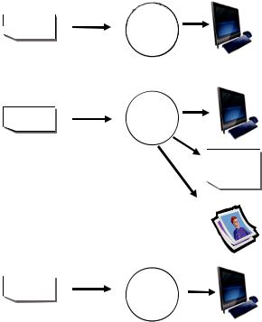
Let’s put it all together with an example. Assume that you have three script files containing R code (script1.R, script2.R, and script3.R). Issuing the statement
source("script1.R")
submits the R code from script1.R to the current session, and the results appear on the screen.
If you then issue the statements
sink("myoutput", append=TRUE, split=TRUE) pdf("mygraphs.pdf")
source("script2.R")
the R code from file script2.R is submitted, and the results again appear on the screen. In addition, the text output is appended to the file myoutput, and the graphic output is saved to the file mygraphs.pdf.
Finally, if you issue the statements
sink()
dev.off()
source("script3.R")
the R code from script3.R is submitted, and the results appear on the screen. This time, no text or graphic output is saved to files. The sequence is outlined in figure 1.6.
R provides quite a bit of flexibility and control over where input comes from and where it goes. In section 1.5, you’ll learn how to run a program in batch mode.
Figure 1.6 Input with the source() function and output with the sink() function
|
|
source("script1.R") |
|
|
script1.R |
Current |
|
|
|
session |
|
|
|
sink("myoutput", append=TRUE, split=TRUE) |
|
|
|
source("script2.R") |
|
|
script2.R |
Current |
|
|
|
session |
myoutput |
|
|
|
|
|
|
|
|
|
|
pdf("mygraphs.pdf") |
Output added |
|
|
to the file |
|
sink(), dev.off()
source("script3.R")
script3.R