

Decision trees |
393 |
Next, the prediction equation developed on the df.train dataset is used to classify cases in the df.validate dataset. By default, the predict() function predicts the log odds of having a malignant outcome. By using the type="response" option, the probability of obtaining a malignant classification is returned instead d. In the next line, cases with probabilities greater than 0.5 are classified into the malignant group and cases with probabilities less than or equal to 0.5 are classified as benign.
Finally, a cross-tabulation of actual status and predicted status (called a confusion matrix) is printed e. It shows that 118 cases that were benign were classified as benign, and 76 cases that were malignant were classified as malignant. Ten cases in the df.validate data frame had missing predictor data and could not be included in the evaluation.
The total number of cases correctly classified (also called the accuracy) was (76 + 118) / 200 or 97% in the validation sample. Statistics for evaluating the accuracy of a classification scheme are discussed more fully in section 17.4.
Before moving on, note that three of the predictor variables (sizeUniformity, shapeUniformity, and singleEpithelialCellSize) have coefficients that don’t differ from zero at the p < .10 level. What, if anything, should you do with predictor variables that have nonsignificant coefficients?
In a prediction context, it’s often useful to remove such variables from the final model. This is especially important in situations where a large number of non-infor- mative predictor variables are adding what is essentially noise to the system.
In this case, stepwise logistic regression can be used to generate a smaller model with fewer variables. Predictor variables are added or removed in order to obtain a model with a smaller AIC value. In the current context, you could use
logit.fit.reduced <- step(fit.logit)
to obtain a more parsimonious model. The reduced model excludes the three variables mentioned previously. When used to predict outcomes in the validation dataset, this reduced model makes fewer errors. Try it out.
The next approach we’ll consider involves the creation of decision or classification trees.
17.3 Decision trees
Decision trees are popular in data-mining contexts. They involve creating a set of binary splits on the predictor variables in order to create a tree that can be used to classify new observations into one of two groups. In this section, we’ll look at two types of decision trees: classical trees and conditional inference trees.
17.3.1Classical decision trees
The process of building a classical decision tree starts with a binary outcome variable (benign/malignant in this case) and a set of predictor variables (the nine cytology measurements). The algorithm is as follows:
1Choose the predictor variable that best splits the data into two groups such that the purity (homogeneity) of the outcome in the two groups is maximized (that

394 |
CHAPTER 17 Classification |
is, as many benign cases in one group and malignant cases in the other as possible). If the predictor is continuous, choose a cut-point that maximizes purity for the two groups created. If the predictor variable is categorical (not applicable in this case), combine the categories to obtain two groups with maximum purity.
2Separate the data into these two groups, and continue the process for each subgroup.
3Repeat steps 1 and 2 until a subgroup contains fewer than a minimum number of observations or no splits decrease the impurity beyond a specified threshold.
The subgroups in the final set are called terminal nodes. Each terminal node is classified as one category of the outcome or the other based on the most frequent value of the outcome for the sample in that node.
4To classify a case, run it down the tree to a terminal node, and assign it the modal outcome value assigned in step 3.
Unfortunately, this process tends to produce a tree that is too large and suffers from overfitting. As a result, new cases aren’t classified well. To compensate, you can prune back the tree by choosing the tree with the lowest 10-fold cross-validated prediction error. This pruned tree is then used for future predictions.
In R, decision trees can be grown and pruned using the rpart() and prune() functions in the rpart package. The following listing creates a decision tree for classifying the cell data as benign or malignant.
Listing 17.3 Creating a classical decision tree with rpart()
>library(rpart)
>set.seed(1234)
> dtree <- |
rpart(class ~ ., |
data=df.train, method="class", |
b Grows the tree |
|||
|
|
|
parms=list(split="information")) |
|
||
> dtree$cptable |
|
|
|
|
||
|
CP |
nsplit rel error |
xerror |
xstd |
|
|
1 |
0.800000 |
0 |
1.00000 |
1.00000 |
0.06484605 |
|
2 |
0.046875 |
1 |
0.20000 |
0.30625 |
0.04150018 |
|
3 |
0.012500 |
3 |
0.10625 |
0.20625 |
0.03467089 |
|
4 |
0.010000 |
4 |
0.09375 |
0.18125 |
0.03264401 |
|
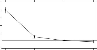
> plotcp(dtree) |
|
|
|
|
> dtree.pruned <- prune(dtree, cp=.0125) |
|
|
|
|
|
|
|
|
|
> library(rpart.plot) |
c Prunes the tree |
|||
|
|
|
|
|
> prp(dtree.pruned, type = 2, extra = 104, |
|
|
|
|
fallen.leaves = TRUE, main="Decision Tree") |
|
|
|
|
> dtree.pred <- predict(dtree.pruned, df.validate, type="class") |
|
Classifies |
||
> dtree.perf <- table(df.validate$class, dtree.pred, |
|
|
|
|
|
|
d new cases |
||
dnn=c("Actual", "Predicted")) |
|
|
||
|
|
|
|
|
> dtree.perf |
|
|
|
|
396 |
CHAPTER 17 Classification |
you can select the tree size associated with the largest complexity parameter below the line in figure 17.1. Results again suggest a tree with three splits (four terminal nodes).
The prune() function uses the complexity parameter to cut back a tree to the desired size. It takes the full tree and snips off the least important splits based on the desired complexity parameter. From the cptable in listing 17.3, a tree with three splits has a complexity parameter of 0.0125, so the statement prune(dtree, cp=0.0125) returns a tree with the desired size c.
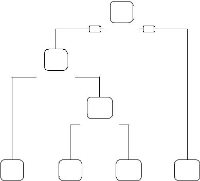
The prp() function in the rpart.plot package is used to draw an attractive plot of the final decision tree (see figure 17.2). The prp() function has many options (see ?prp for details). The type=2 option draws the split labels below each node. The extra=104 parameter includes the probabilities for each class, along with the percentage of observations in each node. The fallen.leaves=TRUE option displays the terminal nodes at the bottom of the graph. To classify an observation, start at the top of the tree, moving to the left branch if a condition is true or to the right otherwise. Continue moving down the tree until you hit a terminal node. Classify the observation using the label of the node.
Decision Tree
benign
.67 .33
100%
yes |
sizeUnif < 3.5 |
no |
benign
.93 .07
71%
bareNucl < 2.5
malignant
.48 .52
9%
shapeUni < 2.5
benign |
benign |
malignant |
malignant |
.99 .01 |
.78 .22 |
.14 .86 |
.05 .95 |
62% |
5% |
4% |
29% |
Figure 17.2 Traditional (pruned) decision tree for predicting cancer status. Start at the top of the tree, moving left if a condition is true or right otherwise. When an observation hits a terminal node, it’s classified. Each node contains the probability of the classes in that node, along with the percentage of the sample.