Figure 3.13 Partial results from demo(plotmath)

to see this in action. A portion of the results is presented in figure 3.13. The plotmath() function can be used to add mathematical symbols to titles, axis labels, or text annotations in the body or margins of a graph.

You can often gain greater insight into your data by comparing several graphs at one time. So, we’ll end this chapter by looking at ways to combine more than one graph into a single image.

3.5Combining graphs

R makes it easy to combine several graphs into one overall graph, using either the par() or layout() function. At this point, don’t worry about the specific types of graphs being combined; our focus here is on the general methods used to combine them. The creation and interpretation of each graph type are covered in later chapters.

With the par() function, you can include the graphical parameter mfrow=c(nrows, ncols) to create a matrix of nrows × ncols plots that are filled in by row. Alternatively, you can use mfcol=c(nrows, ncols) to fill the matrix by columns.

For example, the following code creates four plots and arranges them into two rows and two columns:

attach(mtcars)

opar <- par(no.readonly=TRUE) par(mfrow=c(2,2))

plot(wt,mpg, main="Scatterplot of wt vs. mpg") plot(wt,disp, main="Scatterplot of wt vs. disp") hist(wt, main="Histogram of wt")

boxplot(wt, main="Boxplot of wt") par(opar)

detach(mtcars)

The results are presented in figure 3.14.

As a second example, let’s arrange three plots in three rows and one column. Here’s the code:

attach(mtcars)

opar <- par(no.readonly=TRUE) par(mfrow=c(3,1))

hist(wt)

hist(mpg)

hist(disp)

par(opar)

detach(mtcars)

wt

Figure 3.14 Graph combining four figures through par(mfrow=c(2,2))

66 CHAPTER 3 Getting started with graphs

The graph is displayed in figure 3.15. Note that the high-level function hist() includes a default title (use main="" to suppress it, or ann=FALSE to suppress all titles and labels).

The layout() function has the form layout(mat), where mat is a matrix object specifying the location of the multiple plots to combine. In the following code, one figure is placed in row 1 and two figures are placed in row 2:

attach(mtcars)

layout(matrix(c(1,1,2,3), 2, 2, byrow = TRUE)) hist(wt)

hist(mpg)

hist(disp)

detach(mtcars)

The resulting graph is presented in figure 3.16.

Histogram of wt

wt

Histogram of mpg

mpg

Histogram of disp

disp

Figure 3.15 Graph combining three figures through par(mfrow=c(3,1))

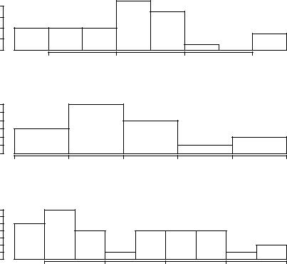
Figure 3.16 Graph combining three figures using the layout() function with default widths

Optionally, you can include widths= and heights= options in the layout() function to control the size of each figure more precisely. These options have the following form:

■widths—A vector of values for the widths of columns

■heights—A vector of values for the heights of rows

Relative widths are specified with numeric values. Absolute widths (in centimeters) are specified with the lcm() function.

In the following code, one figure is again placed in row 1 and two figures are placed in row 2. But the figure in row 1 is one-third the height of the figures in row 2. Additionally, the figure in the bottom-right cell is one-fourth the width of the figure in the bottom-left cell:

attach(mtcars)

layout(matrix(c(1, 1, 2, 3), 2, 2, byrow = TRUE), widths=c(3, 1), heights=c(1, 2))

hist(wt)

hist(mpg)

hist(disp)

detach(mtcars)