

Numerical and character functions |
91 |
5.2Numerical and character functions
In this section, we’ll review functions in R that can be used as the basic building blocks for manipulating data. They can be divided into numerical (mathematical, statistical, probability) and character functions. After we review each type, I’ll show you how to apply functions to the columns (variables) and rows (observations) of matrices and data frames (see section 5.2.6).
5.2.1Mathematical functions
Table 5.2 lists common mathematical functions along with short examples.
Table 5.2 Mathematical functions
Function |
Description |
|
|
abs(x) |
Absolute value |
|
abs(-4) returns 4. |
sqrt(x) |
Square root |
|
sqrt(25) returns 5. This is the same as 25^(0.5). |
ceiling(x) |
Smallest integer not less than x |
|
ceiling(3.475) returns 4. |
floor(x) |
Largest integer not greater than x |
|
floor(3.475) returns 3. |
trunc(x) |
Integer formed by truncating values in x toward 0 |
|
trunc(5.99) returns 5. |
round(x, digits=n) |
Rounds x to the specified number of decimal places |
|
round(3.475, digits=2) returns 3.48. |
signif(x, digits=n) |
Rounds x to the specified number of significant digits |
|
signif(3.475, digits=2) returns 3.5. |
cos(x), sin(x), tan(x) |
Cosine, sine, and tangent |
|
cos(2) returns –0.416. |
acos(x), asin(x), atan(x) |
Arc-cosine, arc-sine, and arc-tangent |
|
acos(-0.416) returns 2. |
cosh(x), sinh(x), tanh(x) |
Hyperbolic cosine, sine, and tangent |
|
sinh(2) returns 3.627. |
acosh(x), asinh(x), atanh(x) |
Hyperbolic arc-cosine, arc-sine, and arc-tangent |
|
asinh(3.627) returns 2. |
log(x,base=n) |
Logarithm of x to the base n |
log(x) |
For convenience: |
log10(x) |
■ log(x) is the natural logarithm. |
|
■ log10(x) is the common logarithm. |
|
■ log(10) returns 2.3026. |
|
■ log10(10) returns 1. |
exp(x) |
Exponential function |
|
exp(2.3026) returns 10. |
|
|
92 |
CHAPTER 5 Advanced data management |
Data transformation is one of the primary uses for these functions. For example, you often transform positively skewed variables such as income to a log scale before further analyses. Mathematical functions are also used as components in formulas, in plotting functions (for example, x versus sin(x)), and in formatting numerical values prior to printing.
The examples in table 5.2 apply mathematical functions to scalars (individual numbers). When these functions are applied to numeric vectors, matrices, or data frames, they operate on each individual value. For example, sqrt(c(4, 16, 25)) returns c(2, 4, 5).
5.2.2Statistical functions
Common statistical functions are presented in table 5.3. Many of these functions have optional parameters that affect the outcome. For example,
y <- mean(x)
provides the arithmetic mean of the elements in object x, and
z <- mean(x, trim = 0.05, na.rm=TRUE)
provides the trimmed mean, dropping the highest and lowest 5% of scores and any missing values. Use the help() function to learn more about each function and its arguments.
Table 5.3 Statistical functions
Function |
Description |
|
|
mean(x) |
Mean |
|
mean(c(1,2,3,4)) returns 2.5. |
median(x) |
Median |
|
median(c(1,2,3,4)) returns 2.5. |
sd(x) |
Standard deviation |
|
sd(c(1,2,3,4)) returns 1.29. |
var(x) |
Variance |
|
var(c(1,2,3,4)) returns 1.67. |
mad(x) |
Median absolute deviation |
|
mad(c(1,2,3,4)) returns 1.48. |
quantile(x, |
Quantiles where x is the numeric vector, where quantiles are desired and |
probs) |
probs is a numeric vector with probabilities in [0,1] |
|
# 30th and 84th percentiles of x |
|
y <- quantile(x, c(.3,.84)) |
range(x) |
Range |
|
x <- c(1,2,3,4) |
|
range(x) returns c(1,4). |
|
diff(range(x)) returns 3. |
sum(x) |
Sum |
|
sum(c(1,2,3,4)) returns 10. |
|
|

Numerical and character functions |
93 |
Table 5.3 Statistical functions
Function |
Description |
|
|
diff(x, lag=n) |
Lagged differences, with lag indicating which lag to use. The default lag is 1. |
|
x<- c(1, 5, 23, 29) |
|
diff(x) returns c(4, 18, 6). |
min(x) |
Minimum |
|
min(c(1,2,3,4)) returns 1. |
max(x) |
Maximum |
|
max(c(1,2,3,4)) returns 4. |
scale(x, |
Column center (center=TRUE) or standardize (center=TRUE, |
center=TRUE, |
scale=TRUE) data object x. An example is given in listing 5.6. |
scale=TRUE) |
|
|
|
To see these functions in action, look at the next listing. This example demonstrates two ways to calculate the mean and standard deviation of a vector of numbers.
Listing 5.1 Calculating the mean and standard deviation
>x <- c(1,2,3,4,5,6,7,8)
>mean(x)
[1] 4.5 > sd(x)
[1] 2.449490
>n <- length(x)
>meanx <- sum(x)/n
>css <- sum((x - meanx)^2)
>sdx <- sqrt(css / (n-1))
>meanx
[1] |
4.5 |
> sdx |
|
[1] |
2.449490 |
Short way
Long way
It’s instructive to view how the corrected sum of squares (css) is calculated in the second approach:
1x equals c(1, 2, 3, 4, 5, 6, 7, 8), and mean x equals 4.5 (length(x) returns the number of elements in x).
2(x – meanx) subtracts 4.5 from each element of x, resulting in
c(-3.5, -2.5, -1.5, -0.5, 0.5, 1.5, 2.5, 3.5)
3 (x – meanx)^2 squares each element of (x - meanx), resulting in
c(12.25, 6.25, 2.25, 0.25, 0.25, 2.25, 6.25, 12.25)
4 sum((x - meanx)^2) sums each of the elements of (x - meanx)^2), resulting in 42.
Writing formulas in R has much in common with matrix-manipulation languages such as MATLAB (we’ll look more specifically at solving matrix algebra problems in appendix D).

94 |
CHAPTER 5 Advanced data management |
Standardizing data
By default, the scale() function standardizes the specified columns of a matrix or data frame to a mean of 0 and a standard deviation of 1:
newdata <- scale(mydata)
To standardize each column to an arbitrary mean and standard deviation, you can use code similar to the following
newdata <- scale(mydata)*SD + M
where M is the desired mean and SD is the desired standard deviation. Using the scale() function on non-numeric columns produces an error. To standardize a specific column rather than an entire matrix or data frame, you can use code such as this:
newdata <- transform(mydata, myvar = scale(myvar)*10+50)
This code standardizes the variable myvar to a mean of 50 and standard deviation of 10. You’ll use the scale() function in the solution to the data-management challenge in section 5.3.
5.2.3Probability functions
You may wonder why probability functions aren’t listed with the statistical functions (it was really bothering you, wasn’t it?). Although probability functions are statistical by definition, they’re unique enough to deserve their own section. Probability functions are often used to generate simulated data with known characteristics and to calculate probability values within user-written statistical functions.
In R, probability functions take the form
[dpqr]distribution_abbreviation()
where the first letter refers to the aspect of the distribution returned:
d = density
p= distribution function
q= quantile function
r= random generation (random deviates)
The common probability functions are listed in table 5.4.
Table 5.4 Probability distributions
Distribution |
Abbreviation |
Distribution |
Abbreviation |
|
|
|
|
Beta |
beta |
Logistic |
logis |
Binomial |
binom |
Multinomial |
multinom |
Cauchy |
cauchy |
Negative binomial |
nbinom |
Chi-squared (noncentral) |
chisq |
Normal |
norm |
Exponential |
exp |
Poisson |
pois |
|
|
|
|
|
Numerical and character functions |
95 |
||
Table 5.4 Probability distributions |
|
|
||
|
|
|
|
|
Distribution |
|
Abbreviation |
Distribution |
Abbreviation |
|
|
|
|
|
F |
|
f |
Wilcoxon signed rank |
signrank |
Gamma |
|
gamma |
T |
t |
Geometric |
|
geom |
Uniform |
unif |
Hypergeometric |
|
hyper |
Weibull |
weibull |
Lognormal |
|
lnorm |
Wilcoxon rank sum |
wilcox |
|
|
|
|
|
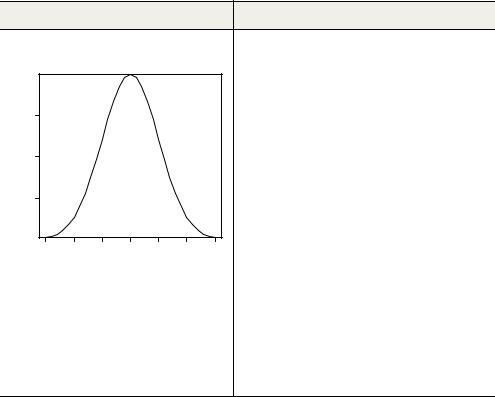
To see how these work, let’s look at functions related to the normal distribution. If you don’t specify a mean and a standard deviation, the standard normal distribution is assumed (mean=0, sd=1). Examples of the density (dnorm), distribution (pnorm), quantile (qnorm), and random deviate generation (rnorm) functions are given in table 5.5.
Table 5.5 Normal distribution functions
|
|
|
Problem |
|
|
|
Solution |
|
Plot the standard normal curve on the interval |
x <- pretty(c(-3,3), 30) |
|||||||
[–3,3] (see figure). |
|
|
|
|
|
y <- dnorm(x) |
||
|
|
|
|
|
|
|
|
plot(x, y, |
|
|
|
|
|
|
|
|
type = "l", |
|
|
|
|
|
|
|
|
xlab = "Normal Deviate", |
|
0.3 |
|
|
|
|
|
|
ylab = "Density", |
|
|
|
|
|
|
|
yaxs = "i" |
|
|
|
|
|
|
|
|
|
|
Density |
|
|
|
|
|
|
|
) |
0.2 |
|
|
|
|
|
|
|
|
|
0.1 |
|
|
|
|
|
|
|
|
−3 |
−2 |
−1 |
0 |
1 |
2 |
3 |
|
Normal Deviate
What is the area under the standard normal |
pnorm(1.96)equals 0.975. |
curve to the left of z=1.96? |
|
What is the value of the 90th percentile of a qnorm(.9, mean=500, sd=100) equals 628.16. normal distribution with a mean of 500 and a
standard deviation of 100?
Generate 50 random normal deviates with a |
rnorm(50, mean=50, sd=10) |
mean of 50 and a standard deviation of 10. |
|
Don’t worry if the plot() function options are unfamiliar. They’re covered in detail in chapter 11; pretty() is explained in table 5.7 later in this chapter.

96 |
CHAPTER 5 Advanced data management |
SETTING THE SEED FOR RANDOM NUMBER GENERATION
Each time you generate pseudo-random deviates, a different seed, and therefore different results, are produced. To make your results reproducible, you can specify the seed explicitly, using the set.seed() function. An example is given in the next listing. Here, the runif() function is used to generate pseudo-random numbers from a uniform distribution on the interval 0 to 1.
Listing 5.2 Generating pseudo-random numbers from a uniform distribution
> runif(5)
[1] 0.8725344 0.3962501 0.6826534 0.3667821 0.9255909 > runif(5)
[1] 0.4273903 0.2641101 0.3550058 0.3233044 0.6584988
>set.seed(1234)
>runif(5)
[1] 0.1137034 0.6222994 0.6092747 0.6233794 0.8609154
>set.seed(1234)
>runif(5)
[1] 0.1137034 0.6222994 0.6092747 0.6233794 0.8609154
By setting the seed manually, you’re able to reproduce your results. This ability can be helpful in creating examples you can access in the future and share with others.
GENERATING MULTIVARIATE NORMAL DATA
In simulation research and Monte Carlo studies, you often want to draw data from a multivariate normal distribution with a given mean vector and covariance matrix. The mvrnorm() function in the MASS package makes this easy. The function call is
mvrnorm(n, mean, sigma)
where n is the desired sample size, mean is the vector of means, and sigma is the vari- ance-covariance (or correlation) matrix. Listing 5.3 samples 500 observations from a three-variable multivariate normal distribution for which the following are true:
Mean vector |
230.7 |
146.7 |
3.6 |
Covariance matrix |
15360.8 |
6721.2 |
-47.1 |
|
6721.2 |
4700.9 |
-16.5 |
|
-47.1 |
-16.5 |
0.3 |
|
|
|
|
Listing 5.3 Generating data from a multivariate normal distribution
> library(MASS) |
b Sets the random number seed |
||
> |
options(digits=3) |
||
> |
set.seed(1234) |
|
|
|
|
||
>mean <- c(230.7, 146.7, 3.6)
>sigma <- matrix(c(15360.8, 6721.2, -47.1,
6721.2, 4700.9, -16.5,
-47.1, -16.5, 0.3), nrow=3, ncol=3)
c Specifies the mean vector and covariance matrix