- •brief contents
- •contents
- •preface
- •acknowledgments
- •about this book
- •What’s new in the second edition
- •Who should read this book
- •Roadmap
- •Advice for data miners
- •Code examples
- •Code conventions
- •Author Online
- •About the author
- •about the cover illustration
- •1 Introduction to R
- •1.2 Obtaining and installing R
- •1.3 Working with R
- •1.3.1 Getting started
- •1.3.2 Getting help
- •1.3.3 The workspace
- •1.3.4 Input and output
- •1.4 Packages
- •1.4.1 What are packages?
- •1.4.2 Installing a package
- •1.4.3 Loading a package
- •1.4.4 Learning about a package
- •1.5 Batch processing
- •1.6 Using output as input: reusing results
- •1.7 Working with large datasets
- •1.8 Working through an example
- •1.9 Summary
- •2 Creating a dataset
- •2.1 Understanding datasets
- •2.2 Data structures
- •2.2.1 Vectors
- •2.2.2 Matrices
- •2.2.3 Arrays
- •2.2.4 Data frames
- •2.2.5 Factors
- •2.2.6 Lists
- •2.3 Data input
- •2.3.1 Entering data from the keyboard
- •2.3.2 Importing data from a delimited text file
- •2.3.3 Importing data from Excel
- •2.3.4 Importing data from XML
- •2.3.5 Importing data from the web
- •2.3.6 Importing data from SPSS
- •2.3.7 Importing data from SAS
- •2.3.8 Importing data from Stata
- •2.3.9 Importing data from NetCDF
- •2.3.10 Importing data from HDF5
- •2.3.11 Accessing database management systems (DBMSs)
- •2.3.12 Importing data via Stat/Transfer
- •2.4 Annotating datasets
- •2.4.1 Variable labels
- •2.4.2 Value labels
- •2.5 Useful functions for working with data objects
- •2.6 Summary
- •3 Getting started with graphs
- •3.1 Working with graphs
- •3.2 A simple example
- •3.3 Graphical parameters
- •3.3.1 Symbols and lines
- •3.3.2 Colors
- •3.3.3 Text characteristics
- •3.3.4 Graph and margin dimensions
- •3.4 Adding text, customized axes, and legends
- •3.4.1 Titles
- •3.4.2 Axes
- •3.4.3 Reference lines
- •3.4.4 Legend
- •3.4.5 Text annotations
- •3.4.6 Math annotations
- •3.5 Combining graphs
- •3.5.1 Creating a figure arrangement with fine control
- •3.6 Summary
- •4 Basic data management
- •4.1 A working example
- •4.2 Creating new variables
- •4.3 Recoding variables
- •4.4 Renaming variables
- •4.5 Missing values
- •4.5.1 Recoding values to missing
- •4.5.2 Excluding missing values from analyses
- •4.6 Date values
- •4.6.1 Converting dates to character variables
- •4.6.2 Going further
- •4.7 Type conversions
- •4.8 Sorting data
- •4.9 Merging datasets
- •4.9.1 Adding columns to a data frame
- •4.9.2 Adding rows to a data frame
- •4.10 Subsetting datasets
- •4.10.1 Selecting (keeping) variables
- •4.10.2 Excluding (dropping) variables
- •4.10.3 Selecting observations
- •4.10.4 The subset() function
- •4.10.5 Random samples
- •4.11 Using SQL statements to manipulate data frames
- •4.12 Summary
- •5 Advanced data management
- •5.2 Numerical and character functions
- •5.2.1 Mathematical functions
- •5.2.2 Statistical functions
- •5.2.3 Probability functions
- •5.2.4 Character functions
- •5.2.5 Other useful functions
- •5.2.6 Applying functions to matrices and data frames
- •5.3 A solution for the data-management challenge
- •5.4 Control flow
- •5.4.1 Repetition and looping
- •5.4.2 Conditional execution
- •5.5 User-written functions
- •5.6 Aggregation and reshaping
- •5.6.1 Transpose
- •5.6.2 Aggregating data
- •5.6.3 The reshape2 package
- •5.7 Summary
- •6 Basic graphs
- •6.1 Bar plots
- •6.1.1 Simple bar plots
- •6.1.2 Stacked and grouped bar plots
- •6.1.3 Mean bar plots
- •6.1.4 Tweaking bar plots
- •6.1.5 Spinograms
- •6.2 Pie charts
- •6.3 Histograms
- •6.4 Kernel density plots
- •6.5 Box plots
- •6.5.1 Using parallel box plots to compare groups
- •6.5.2 Violin plots
- •6.6 Dot plots
- •6.7 Summary
- •7 Basic statistics
- •7.1 Descriptive statistics
- •7.1.1 A menagerie of methods
- •7.1.2 Even more methods
- •7.1.3 Descriptive statistics by group
- •7.1.4 Additional methods by group
- •7.1.5 Visualizing results
- •7.2 Frequency and contingency tables
- •7.2.1 Generating frequency tables
- •7.2.2 Tests of independence
- •7.2.3 Measures of association
- •7.2.4 Visualizing results
- •7.3 Correlations
- •7.3.1 Types of correlations
- •7.3.2 Testing correlations for significance
- •7.3.3 Visualizing correlations
- •7.4 T-tests
- •7.4.3 When there are more than two groups
- •7.5 Nonparametric tests of group differences
- •7.5.1 Comparing two groups
- •7.5.2 Comparing more than two groups
- •7.6 Visualizing group differences
- •7.7 Summary
- •8 Regression
- •8.1 The many faces of regression
- •8.1.1 Scenarios for using OLS regression
- •8.1.2 What you need to know
- •8.2 OLS regression
- •8.2.1 Fitting regression models with lm()
- •8.2.2 Simple linear regression
- •8.2.3 Polynomial regression
- •8.2.4 Multiple linear regression
- •8.2.5 Multiple linear regression with interactions
- •8.3 Regression diagnostics
- •8.3.1 A typical approach
- •8.3.2 An enhanced approach
- •8.3.3 Global validation of linear model assumption
- •8.3.4 Multicollinearity
- •8.4 Unusual observations
- •8.4.1 Outliers
- •8.4.3 Influential observations
- •8.5 Corrective measures
- •8.5.1 Deleting observations
- •8.5.2 Transforming variables
- •8.5.3 Adding or deleting variables
- •8.5.4 Trying a different approach
- •8.6 Selecting the “best” regression model
- •8.6.1 Comparing models
- •8.6.2 Variable selection
- •8.7 Taking the analysis further
- •8.7.1 Cross-validation
- •8.7.2 Relative importance
- •8.8 Summary
- •9 Analysis of variance
- •9.1 A crash course on terminology
- •9.2 Fitting ANOVA models
- •9.2.1 The aov() function
- •9.2.2 The order of formula terms
- •9.3.1 Multiple comparisons
- •9.3.2 Assessing test assumptions
- •9.4 One-way ANCOVA
- •9.4.1 Assessing test assumptions
- •9.4.2 Visualizing the results
- •9.6 Repeated measures ANOVA
- •9.7 Multivariate analysis of variance (MANOVA)
- •9.7.1 Assessing test assumptions
- •9.7.2 Robust MANOVA
- •9.8 ANOVA as regression
- •9.9 Summary
- •10 Power analysis
- •10.1 A quick review of hypothesis testing
- •10.2 Implementing power analysis with the pwr package
- •10.2.1 t-tests
- •10.2.2 ANOVA
- •10.2.3 Correlations
- •10.2.4 Linear models
- •10.2.5 Tests of proportions
- •10.2.7 Choosing an appropriate effect size in novel situations
- •10.3 Creating power analysis plots
- •10.4 Other packages
- •10.5 Summary
- •11 Intermediate graphs
- •11.1 Scatter plots
- •11.1.3 3D scatter plots
- •11.1.4 Spinning 3D scatter plots
- •11.1.5 Bubble plots
- •11.2 Line charts
- •11.3 Corrgrams
- •11.4 Mosaic plots
- •11.5 Summary
- •12 Resampling statistics and bootstrapping
- •12.1 Permutation tests
- •12.2 Permutation tests with the coin package
- •12.2.2 Independence in contingency tables
- •12.2.3 Independence between numeric variables
- •12.2.5 Going further
- •12.3 Permutation tests with the lmPerm package
- •12.3.1 Simple and polynomial regression
- •12.3.2 Multiple regression
- •12.4 Additional comments on permutation tests
- •12.5 Bootstrapping
- •12.6 Bootstrapping with the boot package
- •12.6.1 Bootstrapping a single statistic
- •12.6.2 Bootstrapping several statistics
- •12.7 Summary
- •13 Generalized linear models
- •13.1 Generalized linear models and the glm() function
- •13.1.1 The glm() function
- •13.1.2 Supporting functions
- •13.1.3 Model fit and regression diagnostics
- •13.2 Logistic regression
- •13.2.1 Interpreting the model parameters
- •13.2.2 Assessing the impact of predictors on the probability of an outcome
- •13.2.3 Overdispersion
- •13.2.4 Extensions
- •13.3 Poisson regression
- •13.3.1 Interpreting the model parameters
- •13.3.2 Overdispersion
- •13.3.3 Extensions
- •13.4 Summary
- •14 Principal components and factor analysis
- •14.1 Principal components and factor analysis in R
- •14.2 Principal components
- •14.2.1 Selecting the number of components to extract
- •14.2.2 Extracting principal components
- •14.2.3 Rotating principal components
- •14.2.4 Obtaining principal components scores
- •14.3 Exploratory factor analysis
- •14.3.1 Deciding how many common factors to extract
- •14.3.2 Extracting common factors
- •14.3.3 Rotating factors
- •14.3.4 Factor scores
- •14.4 Other latent variable models
- •14.5 Summary
- •15 Time series
- •15.1 Creating a time-series object in R
- •15.2 Smoothing and seasonal decomposition
- •15.2.1 Smoothing with simple moving averages
- •15.2.2 Seasonal decomposition
- •15.3 Exponential forecasting models
- •15.3.1 Simple exponential smoothing
- •15.3.3 The ets() function and automated forecasting
- •15.4 ARIMA forecasting models
- •15.4.1 Prerequisite concepts
- •15.4.2 ARMA and ARIMA models
- •15.4.3 Automated ARIMA forecasting
- •15.5 Going further
- •15.6 Summary
- •16 Cluster analysis
- •16.1 Common steps in cluster analysis
- •16.2 Calculating distances
- •16.3 Hierarchical cluster analysis
- •16.4 Partitioning cluster analysis
- •16.4.2 Partitioning around medoids
- •16.5 Avoiding nonexistent clusters
- •16.6 Summary
- •17 Classification
- •17.1 Preparing the data
- •17.2 Logistic regression
- •17.3 Decision trees
- •17.3.1 Classical decision trees
- •17.3.2 Conditional inference trees
- •17.4 Random forests
- •17.5 Support vector machines
- •17.5.1 Tuning an SVM
- •17.6 Choosing a best predictive solution
- •17.7 Using the rattle package for data mining
- •17.8 Summary
- •18 Advanced methods for missing data
- •18.1 Steps in dealing with missing data
- •18.2 Identifying missing values
- •18.3 Exploring missing-values patterns
- •18.3.1 Tabulating missing values
- •18.3.2 Exploring missing data visually
- •18.3.3 Using correlations to explore missing values
- •18.4 Understanding the sources and impact of missing data
- •18.5 Rational approaches for dealing with incomplete data
- •18.6 Complete-case analysis (listwise deletion)
- •18.7 Multiple imputation
- •18.8 Other approaches to missing data
- •18.8.1 Pairwise deletion
- •18.8.2 Simple (nonstochastic) imputation
- •18.9 Summary
- •19 Advanced graphics with ggplot2
- •19.1 The four graphics systems in R
- •19.2 An introduction to the ggplot2 package
- •19.3 Specifying the plot type with geoms
- •19.4 Grouping
- •19.5 Faceting
- •19.6 Adding smoothed lines
- •19.7 Modifying the appearance of ggplot2 graphs
- •19.7.1 Axes
- •19.7.2 Legends
- •19.7.3 Scales
- •19.7.4 Themes
- •19.7.5 Multiple graphs per page
- •19.8 Saving graphs
- •19.9 Summary
- •20 Advanced programming
- •20.1 A review of the language
- •20.1.1 Data types
- •20.1.2 Control structures
- •20.1.3 Creating functions
- •20.2 Working with environments
- •20.3 Object-oriented programming
- •20.3.1 Generic functions
- •20.3.2 Limitations of the S3 model
- •20.4 Writing efficient code
- •20.5 Debugging
- •20.5.1 Common sources of errors
- •20.5.2 Debugging tools
- •20.5.3 Session options that support debugging
- •20.6 Going further
- •20.7 Summary
- •21 Creating a package
- •21.1 Nonparametric analysis and the npar package
- •21.1.1 Comparing groups with the npar package
- •21.2 Developing the package
- •21.2.1 Computing the statistics
- •21.2.2 Printing the results
- •21.2.3 Summarizing the results
- •21.2.4 Plotting the results
- •21.2.5 Adding sample data to the package
- •21.3 Creating the package documentation
- •21.4 Building the package
- •21.5 Going further
- •21.6 Summary
- •22 Creating dynamic reports
- •22.1 A template approach to reports
- •22.2 Creating dynamic reports with R and Markdown
- •22.3 Creating dynamic reports with R and LaTeX
- •22.4 Creating dynamic reports with R and Open Document
- •22.5 Creating dynamic reports with R and Microsoft Word
- •22.6 Summary
- •afterword Into the rabbit hole
- •appendix A Graphical user interfaces
- •appendix B Customizing the startup environment
- •appendix C Exporting data from R
- •Delimited text file
- •Excel spreadsheet
- •Statistical applications
- •appendix D Matrix algebra in R
- •appendix E Packages used in this book
- •appendix F Working with large datasets
- •F.1 Efficient programming
- •F.2 Storing data outside of RAM
- •F.3 Analytic packages for out-of-memory data
- •F.4 Comprehensive solutions for working with enormous datasets
- •appendix G Updating an R installation
- •G.1 Automated installation (Windows only)
- •G.2 Manual installation (Windows and Mac OS X)
- •G.3 Updating an R installation (Linux)
- •references
- •index
- •Symbols
- •Numerics
- •23.1 The lattice package
- •23.2 Conditioning variables
- •23.3 Panel functions
- •23.4 Grouping variables
- •23.5 Graphic parameters
- •23.6 Customizing plot strips
- •23.7 Page arrangement
- •23.8 Going further
Working with R |
7 |
■There are some interesting exceptions. Railroad engineers have high income and low education. Ministers have high prestige and low income.
Chapter 8 will have much more to say about this type of graph. The important point is that R allows you to create elegant, informative, highly customized graphs in a simple and straightforward fashion. Creating similar plots in other statistical languages would be difficult, time-consuming, or impossible.
Unfortunately, R can have a steep learning curve. Because it can do so much, the documentation and help files available are voluminous. Additionally, because much of the functionality comes from optional modules created by independent contributors, this documentation can be scattered and difficult to locate. In fact, getting a handle on all that R can do is a challenge.
The goal of this book is to make access to R quick and easy. We’ll tour the many features of R, covering enough material to get you started on your data, with pointers on where to go when you need to learn more. Let’s begin by installing the program.
1.2Obtaining and installing R
R is freely available from the Comprehensive R Archive Network (CRAN) at http:// cran.r-project.org. Precompiled binaries are available for Linux, Mac OS X, and Windows. Follow the directions for installing the base product on the platform of your choice. Later we’ll talk about adding functionality through optional modules called packages (also available from CRAN). Appendix G describes how to update an existing R installation to a newer version.
1.3Working with R
R is a case-sensitive, interpreted language. You can enter commands one at a time at the command prompt (>) or run a set of commands from a source file. There are a wide variety of data types, including vectors, matrices, data frames (similar to datasets), and lists (collections of objects). We’ll discuss each of these data types in chapter 2.
Most functionality is provided through built-in and user-created functions and the creation and manipulation of objects. An object is basically anything that can be assigned a value. For R, that is just about everything (data, functions, graphs, analytic results, and more). Every object has a class attribute telling R how to handle it.
All objects are kept in memory during an interactive session. Basic functions are available by default. Other functions are contained in packages that can be attached to a current session as needed.
Statements consist of functions and assignments. R uses the symbol <- for assignments, rather than the typical = sign. For example, the statement
x <- rnorm(5)
creates a vector object named x containing five random deviates from a standard normal distribution.
8 |
CHAPTER 1 Introduction to R |
NOTE R allows the = sign to be used for object assignments. But you won’t find many programs written that way, because it’s not standard syntax, there are some situations in which it won’t work, and R programmers will make fun of you. You can also reverse the assignment direction. For instance, rnorm(5) -> x is equivalent to the previous statement. Again, doing so is uncommon and isn’t recommended in this book.
Comments are preceded by the # symbol. Any text appearing after the # is ignored by the R interpreter.
1.3.1Getting started
If you’re using Windows, launch R from the Start menu. On a Mac, double-click the R icon in the Applications folder. For Linux, type R at the command prompt of a terminal window. Any of these will start the R interface (see figure 1.3 for an example).
To get a feel for the interface, let’s work through a simple, contrived example. Say that you’re studying physical development and you’ve collected the ages and weights of 10 infants in their first year of life (see table 1.1). You’re interested in the distribution of the weights and their relationship to age.
Figure 1.3 Example of the R interface on Windows
Table 1.1 The ages and weights of 10 infants
Age (mo.) |
Weight (kg.) |
|
|
01 |
4.4 |
03 |
5.3 |
05 |
7.2 |
02 |
5.2 |
11 |
8.5 |
|
|
Age (mo.) |
Weight (kg.) |
|
|
09 |
7.3 |
03 |
6.0 |
09 |
10.4 |
12 |
10.2 |
03 |
6.1 |
|
|
Note: These are fictional data.
Working with R |
9 |
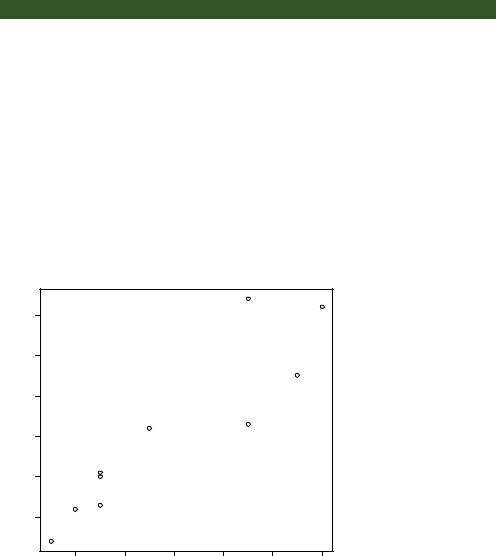
The analysis is given in listing 1.1. Age and weight data are entered as vectors using the function c(), which combines its arguments into a vector or list. The mean and standard deviation of the weights, along with the correlation between age and weight, are provided by the functions mean(), sd(), and cor(), respectively. Finally, age is plotted against weight using the plot() function, allowing you to visually inspect the trend. The q() function ends the session and lets you quit.
Listing 1.1 A sample R session
>age <- c(1,3,5,2,11,9,3,9,12,3)
>weight <- c(4.4,5.3,7.2,5.2,8.5,7.3,6.0,10.4,10.2,6.1)
>mean(weight)
[1] 7.06
>sd(weight) [1] 2.077498
>cor(age,weight) [1] 0.9075655
>plot(age,weight)
>q()
You can see from listing 1.1 that the mean weight for these 10 infants is 7.06 kilograms, that the standard deviation is 2.08 kilograms, and that there is strong linear relationship between age in months and weight in kilograms (correlation = 0.91). The relationship can also be seen in the scatter plot in figure 1.4. Not surprisingly, as infants get older, they tend to weigh more.
weight 5 6 7 8 9 10
2 |
4 |
6 |
8 |
10 |
12 |
age
Figure 1.4 Scatter plot of infant weight (kg) by age (mo)
10 |
CHAPTER 1 Introduction to R |
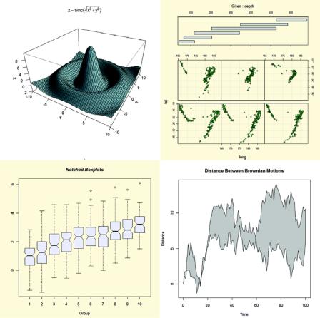
Figure 1.5 A sample of the graphs created with the demo() function
The scatter plot in figure 1.4 is informative but somewhat utilitarian and unattractive. In later chapters, you’ll see how to customize graphs to suit your needs.
TIP To get a sense of what R can do graphically, enter demo()at the command prompt. A sample of the graphs produced is included in figure 1.5. Other demonstrations include demo(Hershey), demo(persp), and demo(image). To see a complete list of demonstrations, enter demo() without parameters.
1.3.2Getting help
R provides extensive help facilities, and learning to navigate them will help you significantly in your programming efforts. The built-in help system provides details, references, and examples of any function contained in a currently installed package. You can obtain help using the functions listed in table 1.2.