


16 |
CHAPTER 1 Introduction to R |
1.4.4Learning about a package
When you load a package, a new set of functions and datasets becomes available. Small illustrative datasets are provided along with sample code, allowing you to try out the new functionalities. The help system contains a description of each function (along with examples) and information about each dataset included. Entering help(package="package_name") provides a brief description of the package and an index of the functions and datasets included. Using help() with any of these function or dataset names provides further details. The same information can be downloaded as a PDF manual from CRAN.
Common mistakes in R programming
Some common mistakes are made frequently by both beginning and experienced R programmers. If your program generates an error, be sure to check for the following:
■Using the wrong case—help(), Help(), and HELP() are three different functions (only the first will work).
■Forgetting to use quotation marks when they’re needed—install.packages- ("gclus") works, whereas install.packages(gclus) generates an error.
■Forgetting to include the parentheses in a function call—For example, help() works, but help doesn’t. Even if there are no options, you still need the ().
■Using the \ in a pathname on Windows—R sees the backslash character as an escape character. setwd("c:\mydata") generates an error. Use setwd("c:/ mydata") or setwd("c:\\mydata") instead.
■Using a function from a package that’s not loaded—The function order.clusters() is contained in the gclus package. If you try to use it before loading the package, you’ll get an error.
The error messages in R can be cryptic, but if you’re careful to follow these points, you should avoid seeing many of them.
1.5Batch processing
Most of the time, you’ll be running R interactively, entering commands at the command prompt and seeing the results of each statement as it’s processed. Occasionally, you may want to run an R program in a repeated, standard, and possibly unattended fashion. For example, you may need to generate the same report once a month. You can write your program in R and run it in batch mode.
How you run R in batch mode depends on your operating system. On Linux or Mac OS X systems, you can use the following command in a terminal window
R CMD BATCH options infile outfile
where infile is the name of the file containing R code to be executed, outfile is the name of the file receiving the output, and options lists options that control execution. By convention, infile is given the extension .R, and outfile is given the extension .Rout.
Working with large datasets |
17 |
For Windows, use
"C:\Program Files\R\R-3.1.0\bin\R.exe" CMD BATCH--vanilla --slave "c:\my projects\myscript.R"
adjusting the paths to match the location of your R.exe binary and your script file. For additional details on how to invoke R, including the use of command-line options, see the “Introduction to R” documentation available from CRAN (http:// cran.r-project.org).
1.6Using output as input: reusing results
One of the most useful design features of R is that the output of analyses can easily be saved and used as input to additional analyses. Let’s walk through an example, using one of the datasets that comes preinstalled with R. If you don’t understand the statistics involved, don’t worry. We’re focusing on the general principle here.
First, run a simple linear regression predicting miles per gallon (mpg) from car weight (wt), using the automotive dataset mtcars. This is accomplished with the following function call:
lm(mpg~wt, data=mtcars)
The results are displayed on the screen, and no information is saved.
Next, run the regression, but store the results in an object:
lmfit <- lm(mpg~wt, data=mtcars)
The assignment creates a list object called lmfit that contains extensive information from the analysis (including the predicted values, residuals, regression coefficients, and more). Although no output is sent to the screen, the results can be both displayed and manipulated further.
Typing summary(lmfit) displays a summary of the results, and plot(lmfit) produces diagnostic plots. The statement cook<-cooks.distance(lmfit) generates and stores influence statistics, and plot(cook) graphs them. To predict miles per gallon from car weight in a new set of data, you’d use predict(lmfit, mynewdata).
To see what a function returns, look at the Value section of the R help page for that function. Here you’d look at help(lm) or ?lm. This tells you what’s saved when you assign the results of that function to an object.
1.7Working with large datasets
Programmers frequently ask me if R can handle large data problems. Typically, they work with massive amounts of data gathered from web research, climatology, or genetics. Because R holds objects in memory, you’re generally limited by the amount of RAM available. For example, on my 5-year-old Windows PC with 2 GB of RAM, I can easily handle datasets with 10 million elements (100 variables by 100,000 observations). On an iMac with 4 GB of RAM, I can usually handle 100 million elements without difficulty.
But there are two issues to consider: the size of the dataset and the statistical methods that will be applied. R can handle data analysis problems in the gigabyte to
18 |
CHAPTER 1 Introduction to R |
terabyte range, but specialized procedures are required. The management and analysis of very large datasets is discussed in appendix F.
1.8Working through an example
We’ll finish this chapter with an example that ties together many of these ideas. Here’s the task:
1Open the general help, and look at the “Introduction to R” section.
2Install the vcd package (a package for visualizing categorical data that you’ll be using in chapter 11).
3List the functions and datasets available in this package.
4Load the package, and read the description of the dataset Arthritis.
5Print out the Arthritis dataset (entering the name of an object will list it).
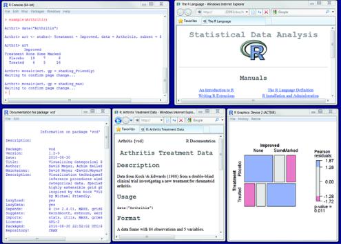
6Run the example that comes with the Arthritis dataset. Don’t worry if you don’t understand the results; it basically shows that arthritis patients receiving treatment improved much more than patients receiving a placebo.
7Quit.
Figure 1.7 Output from listing 1.3, including (left to right) output from the arthritis example, general help, information about the vcd package, information about the Arthritis dataset, and a graph displaying the relationship between arthritis treatment and outcome

Summary |
19 |
The code required is provided in the following listing, with a sample of the results displayed in figure 1.7. As this short exercise demonstrates, you can accomplish a great deal with a small amount of code.
Listing 1.3 Working with a new package
help.start()
install.packages("vcd")
help(package="vcd")
library(vcd)
help(Arthritis) Arthritis example(Arthritis) q()
1.9Summary
In this chapter, we looked at some of the strengths that make R an attractive option for students, researchers, statisticians, and data analysts trying to understand the meaning of their data. We walked through the program’s installation and talked about how to enhance R’s capabilities by downloading additional packages. We explored the basic interface, running programs interactively and in a batch, and produced a few sample graphs. You also learned how to save your work to both text and graphic files. Because R can be a complex program, we spent some time looking at how to access the extensive help that’s available. Hopefully you’re getting a sense of how powerful this freely available software can be.
Now that you have R up and running, it’s time to get your data into the mix. In the next chapter, we’ll look at the types of data R can handle and how to import them into R from text files, other programs, and database management systems.