(continued)

■R doesn’t provide multiline or block comments. You must start each line of a multiline comment with #. For debugging purposes, you can also surround code that you want the interpreter to ignore with the statement if(FALSE){...}. Changing the FALSE to TRUE allows the code to be executed.

■Assigning a value to a nonexistent element of a vector, matrix, array, or list expands that structure to accommodate the new value. For example, consider the following:

>x <- c(8, 6, 4)

>x[7] <- 10

>x

[1]8 6 4 NA NA NA 10

The vector x has expanded from three to seven elements through the assignment. x <- x[1:3] would shrink it back to three elements.

■R doesn’t have scalar values. Scalars are represented as one-element vectors.

■Indices in R start at 1, not at 0. In the vector earlier, x[1] is 8.

■Variables can’t be declared. They come into existence on first assignment.

To learn more, see John Cook’s excellent blog post, “R Language for Programmers” (http://mng.bz/6NwQ). Programmers looking for stylistic guidance may also want to check out “Google’s R Style Guide” (http://mng.bz/i775).

2.3Data input

Now that you have data structures, you need to put some data in them! As a data analyst, you’re typically faced with data that comes from a variety of sources and in a variety of formats. Your task is to import the data into your tools, analyze the data, and report on the results. R provides a wide range of tools for importing data. The definitive guide for importing data in R is the R Data Import/Export manual available at http://mng.bz/urwn.

As you can see in figure 2.2, R can import data from the keyboard, from text files, from Microsoft Excel and Access, from popular statistical packages, from a variety of

SQL MySQL Oracle Access

Figure 2.2 Sources of data that

relational database management systems, from specialty databases, and from web sites and online services. Because you never know where your data will come from, we’ll cover each of them here. You only need to read about the ones you’re going to be using.

2.3.1Entering data from the keyboard

Perhaps the simplest way to enter data is from the keyboard. There are two common methods: entering data through R’s built-in text editor and embedding data directly into your code. We’ll consider the editor first.

The edit() function in R invokes a text editor that lets you enter data manually. Here are the steps:

1Create an empty data frame (or matrix) with the variable names and modes you want to have in the final dataset.

2Invoke the text editor on this data object, enter your data, and save the results to the data object.

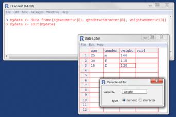
The following example creates a data frame named mydata with three variables: age (numeric), gender (character), and weight (numeric). You then invoke the text editor, add your data, and save the results:

mydata <- data.frame(age=numeric(0), gender=character(0), weight=numeric(0))

mydata <- edit(mydata)

Assignments like age=numeric(0) create a variable of a specific mode, but without actual data. Note that the result of the editing is assigned back to the object itself. The edit() function operates on a copy of the object. If you don’t assign it a destination, all of your edits will be lost!

The results of invoking the edit() function on a Windows platform are shown in figure 2.3. In this figure, I’ve added some data. If you click a column title, the editor

Figure 2.3 Entering data via the built-in editor on a Windows platform

gives you the option of changing the variable name and type (numeric or character). You can add variables by clicking the titles of unused columns. When the text editor is closed, the results are saved to the object assigned (mydata, in this case). Invoking mydata <- edit(mydata) again allows you to edit the data you’ve entered and to add new data. A shortcut for mydata <- edit(mydata) is fix(mydata).

Alternatively, you can embed the data directly in your program. For example, the code

mydatatxt <- " age gender weight 25 m 166

30 f 115

18 f 120

"

mydata <- read.table(header=TRUE, text=mydatatxt)

creates the same data frame as that created with the edit() function. A character string is created containing the raw data, and the read.table() function is used to process the string and return a data frame. The read.table() function is described more fully in the next section.

Keyboard data entry can be convenient when you’re working with small datasets. For larger datasets, you’ll want to use the methods described next: importing data from existing text files, Excel spreadsheets, statistical packages, or databasemanagement systems.

2.3.2Importing data from a delimited text file

You can import data from delimited text files using read.table(), a function that reads a file in table format and saves it as a data frame. Each row of the table appears as one line in the file. The syntax is

mydataframe <- read.table(file, options)

where file is a delimited ASCII file and the options are parameters controlling how data is processed. The most common options are listed in table 2.2.

Table 2.2 read.table() options

There are several interesting things to note about how the data is imported. The variable name Social Studies is automatically renamed to follow R conventions. The StudentID column is now the row name, no longer has a label, and has lost its leading zero. The missing science grade for Jane is correctly read as missing. I had to put quotation marks around Dan's last name in order to escape the comma between Thornton and III. Otherwise, R would have seen seven values on that line, rather than six. I also had to put quotation marks around O'Leary. Otherwise, R would have read the single quote as a string delimiter (which isn’t what I want). Finally, the first and last names are converted to factors.

By default, read.table() converts character variables to factors, which may not always be desirable. For example, there would be little reason to convert a character variable containing a respondent’s comments into a factor. You can suppress this behavior in a number of ways. Including the option stringsAsFactors=FALSE turns off this behavior for all character variables. Alternatively, you can use the colClasses option to specify a class (for example, logical, numeric, character, or factor) for each column.

Importing the same data with

grades <- read.table("studentgrades.csv", header=TRUE, row.names="StudentID", sep=",", colClasses=c("character", "character", "character",

"numeric", "numeric", "numeric"))

produces the following data frame:

Note that the row names retain their leading zero and First and Last are no longer factors. Additionally, the grades are stored as real values rather than integers.