

- •brief contents
- •contents
- •preface
- •acknowledgments
- •about this book
- •What’s new in the second edition
- •Who should read this book
- •Roadmap
- •Advice for data miners
- •Code examples
- •Code conventions
- •Author Online
- •About the author
- •about the cover illustration
- •1 Introduction to R
- •1.2 Obtaining and installing R
- •1.3 Working with R
- •1.3.1 Getting started
- •1.3.2 Getting help
- •1.3.3 The workspace
- •1.3.4 Input and output
- •1.4 Packages
- •1.4.1 What are packages?
- •1.4.2 Installing a package
- •1.4.3 Loading a package
- •1.4.4 Learning about a package
- •1.5 Batch processing
- •1.6 Using output as input: reusing results
- •1.7 Working with large datasets
- •1.8 Working through an example
- •1.9 Summary
- •2 Creating a dataset
- •2.1 Understanding datasets
- •2.2 Data structures
- •2.2.1 Vectors
- •2.2.2 Matrices
- •2.2.3 Arrays
- •2.2.4 Data frames
- •2.2.5 Factors
- •2.2.6 Lists
- •2.3 Data input
- •2.3.1 Entering data from the keyboard
- •2.3.2 Importing data from a delimited text file
- •2.3.3 Importing data from Excel
- •2.3.4 Importing data from XML
- •2.3.5 Importing data from the web
- •2.3.6 Importing data from SPSS
- •2.3.7 Importing data from SAS
- •2.3.8 Importing data from Stata
- •2.3.9 Importing data from NetCDF
- •2.3.10 Importing data from HDF5
- •2.3.11 Accessing database management systems (DBMSs)
- •2.3.12 Importing data via Stat/Transfer
- •2.4 Annotating datasets
- •2.4.1 Variable labels
- •2.4.2 Value labels
- •2.5 Useful functions for working with data objects
- •2.6 Summary
- •3 Getting started with graphs
- •3.1 Working with graphs
- •3.2 A simple example
- •3.3 Graphical parameters
- •3.3.1 Symbols and lines
- •3.3.2 Colors
- •3.3.3 Text characteristics
- •3.3.4 Graph and margin dimensions
- •3.4 Adding text, customized axes, and legends
- •3.4.1 Titles
- •3.4.2 Axes
- •3.4.3 Reference lines
- •3.4.4 Legend
- •3.4.5 Text annotations
- •3.4.6 Math annotations
- •3.5 Combining graphs
- •3.5.1 Creating a figure arrangement with fine control
- •3.6 Summary
- •4 Basic data management
- •4.1 A working example
- •4.2 Creating new variables
- •4.3 Recoding variables
- •4.4 Renaming variables
- •4.5 Missing values
- •4.5.1 Recoding values to missing
- •4.5.2 Excluding missing values from analyses
- •4.6 Date values
- •4.6.1 Converting dates to character variables
- •4.6.2 Going further
- •4.7 Type conversions
- •4.8 Sorting data
- •4.9 Merging datasets
- •4.9.1 Adding columns to a data frame
- •4.9.2 Adding rows to a data frame
- •4.10 Subsetting datasets
- •4.10.1 Selecting (keeping) variables
- •4.10.2 Excluding (dropping) variables
- •4.10.3 Selecting observations
- •4.10.4 The subset() function
- •4.10.5 Random samples
- •4.11 Using SQL statements to manipulate data frames
- •4.12 Summary
- •5 Advanced data management
- •5.2 Numerical and character functions
- •5.2.1 Mathematical functions
- •5.2.2 Statistical functions
- •5.2.3 Probability functions
- •5.2.4 Character functions
- •5.2.5 Other useful functions
- •5.2.6 Applying functions to matrices and data frames
- •5.3 A solution for the data-management challenge
- •5.4 Control flow
- •5.4.1 Repetition and looping
- •5.4.2 Conditional execution
- •5.5 User-written functions
- •5.6 Aggregation and reshaping
- •5.6.1 Transpose
- •5.6.2 Aggregating data
- •5.6.3 The reshape2 package
- •5.7 Summary
- •6 Basic graphs
- •6.1 Bar plots
- •6.1.1 Simple bar plots
- •6.1.2 Stacked and grouped bar plots
- •6.1.3 Mean bar plots
- •6.1.4 Tweaking bar plots
- •6.1.5 Spinograms
- •6.2 Pie charts
- •6.3 Histograms
- •6.4 Kernel density plots
- •6.5 Box plots
- •6.5.1 Using parallel box plots to compare groups
- •6.5.2 Violin plots
- •6.6 Dot plots
- •6.7 Summary
- •7 Basic statistics
- •7.1 Descriptive statistics
- •7.1.1 A menagerie of methods
- •7.1.2 Even more methods
- •7.1.3 Descriptive statistics by group
- •7.1.4 Additional methods by group
- •7.1.5 Visualizing results
- •7.2 Frequency and contingency tables
- •7.2.1 Generating frequency tables
- •7.2.2 Tests of independence
- •7.2.3 Measures of association
- •7.2.4 Visualizing results
- •7.3 Correlations
- •7.3.1 Types of correlations
- •7.3.2 Testing correlations for significance
- •7.3.3 Visualizing correlations
- •7.4 T-tests
- •7.4.3 When there are more than two groups
- •7.5 Nonparametric tests of group differences
- •7.5.1 Comparing two groups
- •7.5.2 Comparing more than two groups
- •7.6 Visualizing group differences
- •7.7 Summary
- •8 Regression
- •8.1 The many faces of regression
- •8.1.1 Scenarios for using OLS regression
- •8.1.2 What you need to know
- •8.2 OLS regression
- •8.2.1 Fitting regression models with lm()
- •8.2.2 Simple linear regression
- •8.2.3 Polynomial regression
- •8.2.4 Multiple linear regression
- •8.2.5 Multiple linear regression with interactions
- •8.3 Regression diagnostics
- •8.3.1 A typical approach
- •8.3.2 An enhanced approach
- •8.3.3 Global validation of linear model assumption
- •8.3.4 Multicollinearity
- •8.4 Unusual observations
- •8.4.1 Outliers
- •8.4.3 Influential observations
- •8.5 Corrective measures
- •8.5.1 Deleting observations
- •8.5.2 Transforming variables
- •8.5.3 Adding or deleting variables
- •8.5.4 Trying a different approach
- •8.6 Selecting the “best” regression model
- •8.6.1 Comparing models
- •8.6.2 Variable selection
- •8.7 Taking the analysis further
- •8.7.1 Cross-validation
- •8.7.2 Relative importance
- •8.8 Summary
- •9 Analysis of variance
- •9.1 A crash course on terminology
- •9.2 Fitting ANOVA models
- •9.2.1 The aov() function
- •9.2.2 The order of formula terms
- •9.3.1 Multiple comparisons
- •9.3.2 Assessing test assumptions
- •9.4 One-way ANCOVA
- •9.4.1 Assessing test assumptions
- •9.4.2 Visualizing the results
- •9.6 Repeated measures ANOVA
- •9.7 Multivariate analysis of variance (MANOVA)
- •9.7.1 Assessing test assumptions
- •9.7.2 Robust MANOVA
- •9.8 ANOVA as regression
- •9.9 Summary
- •10 Power analysis
- •10.1 A quick review of hypothesis testing
- •10.2 Implementing power analysis with the pwr package
- •10.2.1 t-tests
- •10.2.2 ANOVA
- •10.2.3 Correlations
- •10.2.4 Linear models
- •10.2.5 Tests of proportions
- •10.2.7 Choosing an appropriate effect size in novel situations
- •10.3 Creating power analysis plots
- •10.4 Other packages
- •10.5 Summary
- •11 Intermediate graphs
- •11.1 Scatter plots
- •11.1.3 3D scatter plots
- •11.1.4 Spinning 3D scatter plots
- •11.1.5 Bubble plots
- •11.2 Line charts
- •11.3 Corrgrams
- •11.4 Mosaic plots
- •11.5 Summary
- •12 Resampling statistics and bootstrapping
- •12.1 Permutation tests
- •12.2 Permutation tests with the coin package
- •12.2.2 Independence in contingency tables
- •12.2.3 Independence between numeric variables
- •12.2.5 Going further
- •12.3 Permutation tests with the lmPerm package
- •12.3.1 Simple and polynomial regression
- •12.3.2 Multiple regression
- •12.4 Additional comments on permutation tests
- •12.5 Bootstrapping
- •12.6 Bootstrapping with the boot package
- •12.6.1 Bootstrapping a single statistic
- •12.6.2 Bootstrapping several statistics
- •12.7 Summary
- •13 Generalized linear models
- •13.1 Generalized linear models and the glm() function
- •13.1.1 The glm() function
- •13.1.2 Supporting functions
- •13.1.3 Model fit and regression diagnostics
- •13.2 Logistic regression
- •13.2.1 Interpreting the model parameters
- •13.2.2 Assessing the impact of predictors on the probability of an outcome
- •13.2.3 Overdispersion
- •13.2.4 Extensions
- •13.3 Poisson regression
- •13.3.1 Interpreting the model parameters
- •13.3.2 Overdispersion
- •13.3.3 Extensions
- •13.4 Summary
- •14 Principal components and factor analysis
- •14.1 Principal components and factor analysis in R
- •14.2 Principal components
- •14.2.1 Selecting the number of components to extract
- •14.2.2 Extracting principal components
- •14.2.3 Rotating principal components
- •14.2.4 Obtaining principal components scores
- •14.3 Exploratory factor analysis
- •14.3.1 Deciding how many common factors to extract
- •14.3.2 Extracting common factors
- •14.3.3 Rotating factors
- •14.3.4 Factor scores
- •14.4 Other latent variable models
- •14.5 Summary
- •15 Time series
- •15.1 Creating a time-series object in R
- •15.2 Smoothing and seasonal decomposition
- •15.2.1 Smoothing with simple moving averages
- •15.2.2 Seasonal decomposition
- •15.3 Exponential forecasting models
- •15.3.1 Simple exponential smoothing
- •15.3.3 The ets() function and automated forecasting
- •15.4 ARIMA forecasting models
- •15.4.1 Prerequisite concepts
- •15.4.2 ARMA and ARIMA models
- •15.4.3 Automated ARIMA forecasting
- •15.5 Going further
- •15.6 Summary
- •16 Cluster analysis
- •16.1 Common steps in cluster analysis
- •16.2 Calculating distances
- •16.3 Hierarchical cluster analysis
- •16.4 Partitioning cluster analysis
- •16.4.2 Partitioning around medoids
- •16.5 Avoiding nonexistent clusters
- •16.6 Summary
- •17 Classification
- •17.1 Preparing the data
- •17.2 Logistic regression
- •17.3 Decision trees
- •17.3.1 Classical decision trees
- •17.3.2 Conditional inference trees
- •17.4 Random forests
- •17.5 Support vector machines
- •17.5.1 Tuning an SVM
- •17.6 Choosing a best predictive solution
- •17.7 Using the rattle package for data mining
- •17.8 Summary
- •18 Advanced methods for missing data
- •18.1 Steps in dealing with missing data
- •18.2 Identifying missing values
- •18.3 Exploring missing-values patterns
- •18.3.1 Tabulating missing values
- •18.3.2 Exploring missing data visually
- •18.3.3 Using correlations to explore missing values
- •18.4 Understanding the sources and impact of missing data
- •18.5 Rational approaches for dealing with incomplete data
- •18.6 Complete-case analysis (listwise deletion)
- •18.7 Multiple imputation
- •18.8 Other approaches to missing data
- •18.8.1 Pairwise deletion
- •18.8.2 Simple (nonstochastic) imputation
- •18.9 Summary
- •19 Advanced graphics with ggplot2
- •19.1 The four graphics systems in R
- •19.2 An introduction to the ggplot2 package
- •19.3 Specifying the plot type with geoms
- •19.4 Grouping
- •19.5 Faceting
- •19.6 Adding smoothed lines
- •19.7 Modifying the appearance of ggplot2 graphs
- •19.7.1 Axes
- •19.7.2 Legends
- •19.7.3 Scales
- •19.7.4 Themes
- •19.7.5 Multiple graphs per page
- •19.8 Saving graphs
- •19.9 Summary
- •20 Advanced programming
- •20.1 A review of the language
- •20.1.1 Data types
- •20.1.2 Control structures
- •20.1.3 Creating functions
- •20.2 Working with environments
- •20.3 Object-oriented programming
- •20.3.1 Generic functions
- •20.3.2 Limitations of the S3 model
- •20.4 Writing efficient code
- •20.5 Debugging
- •20.5.1 Common sources of errors
- •20.5.2 Debugging tools
- •20.5.3 Session options that support debugging
- •20.6 Going further
- •20.7 Summary
- •21 Creating a package
- •21.1 Nonparametric analysis and the npar package
- •21.1.1 Comparing groups with the npar package
- •21.2 Developing the package
- •21.2.1 Computing the statistics
- •21.2.2 Printing the results
- •21.2.3 Summarizing the results
- •21.2.4 Plotting the results
- •21.2.5 Adding sample data to the package
- •21.3 Creating the package documentation
- •21.4 Building the package
- •21.5 Going further
- •21.6 Summary
- •22 Creating dynamic reports
- •22.1 A template approach to reports
- •22.2 Creating dynamic reports with R and Markdown
- •22.3 Creating dynamic reports with R and LaTeX
- •22.4 Creating dynamic reports with R and Open Document
- •22.5 Creating dynamic reports with R and Microsoft Word
- •22.6 Summary
- •afterword Into the rabbit hole
- •appendix A Graphical user interfaces
- •appendix B Customizing the startup environment
- •appendix C Exporting data from R
- •Delimited text file
- •Excel spreadsheet
- •Statistical applications
- •appendix D Matrix algebra in R
- •appendix E Packages used in this book
- •appendix F Working with large datasets
- •F.1 Efficient programming
- •F.2 Storing data outside of RAM
- •F.3 Analytic packages for out-of-memory data
- •F.4 Comprehensive solutions for working with enormous datasets
- •appendix G Updating an R installation
- •G.1 Automated installation (Windows only)
- •G.2 Manual installation (Windows and Mac OS X)
- •G.3 Updating an R installation (Linux)
- •references
- •index
- •Symbols
- •Numerics
- •23.1 The lattice package
- •23.2 Conditioning variables
- •23.3 Panel functions
- •23.4 Grouping variables
- •23.5 Graphic parameters
- •23.6 Customizing plot strips
- •23.7 Page arrangement
- •23.8 Going further
366 |
CHAPTER 15 Time series |
Forecasts from ARIMA(0,1,1)
|
1400 |
|
|
|
|
|
1200 |
|
|
|
|
Flow |
1000 |
|
|
|
|
Annual |
800 |
|
|
|
|
|
600 |
|
|
|
|
|
1880 |
1900 |
1920 |
1940 |
1960 |
|
|
|
Year |
|
|
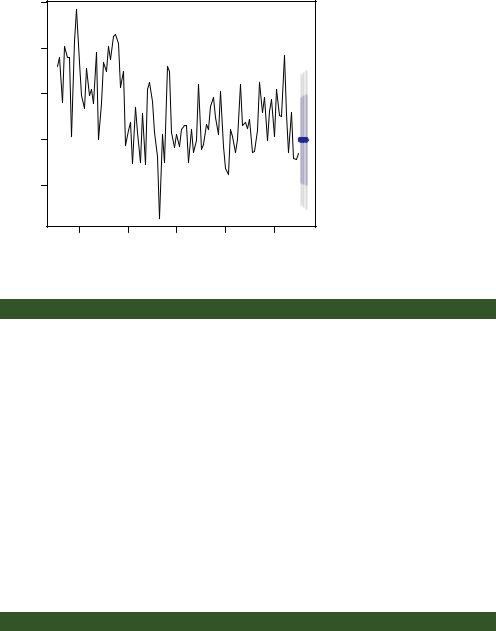
Figure 15.14 Three-year forecast for the Nile time series from a fitted ARIMA(0,1,1) model. Blue dots represent point estimates, and the light and dark gray bands represent the 80% and 95% confidence bands limits, respectively.
Listing 15.10 Forecasting with an ARIMA model
> forecast(fit, 3) |
|
|
|
|
|
|
Point Forecast |
Lo 80 |
Hi 80 |
Lo 95 |
Hi 95 |
1971 |
798.3673 |
614.4307 |
982.3040 |
517.0605 |
1079.674 |
1972 |
798.3673 |
607.9845 |
988.7502 |
507.2019 |
1089.533 |
1973 |
798.3673 |
601.7495 |
994.9851 |
497.6663 |
1099.068 |
> plot(forecast(fit, 3), xlab="Year", ylab="Annual Flow")
The plot() function is used to plot the forecast in figure 15.14. Point estimates are given by the blue dots, and 80% and 95% confidence bands are represented by dark and light bands, respectively.
15.4.3Automated ARIMA forecasting
In section 15.2.3, you used the ets() function in the forecast package to automate the selection of a best exponential model. The package also provides an auto.arima() function to select a best ARIMA model. The next listing applies this approach to the sunspots time series described in the chapter introduction.
Listing 15.11 Automated ARIMA forecasting
>library(forecast)
>fit <- auto.arima(sunspots)
>fit
Series: sunspots
ARIMA(2,1,2)