

- •About the author
- •Brief Contents
- •Contents
- •Preface
- •This Book’s Approach
- •What’s New in the Seventh Edition?
- •The Arrangement of Topics
- •Part One, Introduction
- •Part Two, Classical Theory: The Economy in the Long Run
- •Part Three, Growth Theory: The Economy in the Very Long Run
- •Part Four, Business Cycle Theory: The Economy in the Short Run
- •Part Five, Macroeconomic Policy Debates
- •Part Six, More on the Microeconomics Behind Macroeconomics
- •Epilogue
- •Alternative Routes Through the Text
- •Learning Tools
- •Case Studies
- •FYI Boxes
- •Graphs
- •Mathematical Notes
- •Chapter Summaries
- •Key Concepts
- •Questions for Review
- •Problems and Applications
- •Chapter Appendices
- •Glossary
- •Translations
- •Acknowledgments
- •Supplements and Media
- •For Instructors
- •Instructor’s Resources
- •Solutions Manual
- •Test Bank
- •PowerPoint Slides
- •For Students
- •Student Guide and Workbook
- •Online Offerings
- •EconPortal, Available Spring 2010
- •eBook
- •WebCT
- •BlackBoard
- •Additional Offerings
- •i-clicker
- •The Wall Street Journal Edition
- •Financial Times Edition
- •Dismal Scientist
- •1-1: What Macroeconomists Study
- •1-2: How Economists Think
- •Theory as Model Building
- •The Use of Multiple Models
- •Prices: Flexible Versus Sticky
- •Microeconomic Thinking and Macroeconomic Models
- •1-3: How This Book Proceeds
- •Income, Expenditure, and the Circular Flow
- •Rules for Computing GDP
- •Real GDP Versus Nominal GDP
- •The GDP Deflator
- •Chain-Weighted Measures of Real GDP
- •The Components of Expenditure
- •Other Measures of Income
- •Seasonal Adjustment
- •The Price of a Basket of Goods
- •The CPI Versus the GDP Deflator
- •The Household Survey
- •The Establishment Survey
- •The Factors of Production
- •The Production Function
- •The Supply of Goods and Services
- •3-2: How Is National Income Distributed to the Factors of Production?
- •Factor Prices
- •The Decisions Facing the Competitive Firm
- •The Firm’s Demand for Factors
- •The Division of National Income
- •The Cobb–Douglas Production Function
- •Consumption
- •Investment
- •Government Purchases
- •Changes in Saving: The Effects of Fiscal Policy
- •Changes in Investment Demand
- •3-5: Conclusion
- •4-1: What Is Money?
- •The Functions of Money
- •The Types of Money
- •The Development of Fiat Money
- •How the Quantity of Money Is Controlled
- •How the Quantity of Money Is Measured
- •4-2: The Quantity Theory of Money
- •Transactions and the Quantity Equation
- •From Transactions to Income
- •The Assumption of Constant Velocity
- •Money, Prices, and Inflation
- •4-4: Inflation and Interest Rates
- •Two Interest Rates: Real and Nominal
- •The Fisher Effect
- •Two Real Interest Rates: Ex Ante and Ex Post
- •The Cost of Holding Money
- •Future Money and Current Prices
- •4-6: The Social Costs of Inflation
- •The Layman’s View and the Classical Response
- •The Costs of Expected Inflation
- •The Costs of Unexpected Inflation
- •One Benefit of Inflation
- •4-7: Hyperinflation
- •The Costs of Hyperinflation
- •The Causes of Hyperinflation
- •4-8: Conclusion: The Classical Dichotomy
- •The Role of Net Exports
- •International Capital Flows and the Trade Balance
- •International Flows of Goods and Capital: An Example
- •Capital Mobility and the World Interest Rate
- •Why Assume a Small Open Economy?
- •The Model
- •How Policies Influence the Trade Balance
- •Evaluating Economic Policy
- •Nominal and Real Exchange Rates
- •The Real Exchange Rate and the Trade Balance
- •The Determinants of the Real Exchange Rate
- •How Policies Influence the Real Exchange Rate
- •The Effects of Trade Policies
- •The Special Case of Purchasing-Power Parity
- •Net Capital Outflow
- •The Model
- •Policies in the Large Open Economy
- •Conclusion
- •Causes of Frictional Unemployment
- •Public Policy and Frictional Unemployment
- •Minimum-Wage Laws
- •Unions and Collective Bargaining
- •Efficiency Wages
- •The Duration of Unemployment
- •Trends in Unemployment
- •Transitions Into and Out of the Labor Force
- •6-5: Labor-Market Experience: Europe
- •The Rise in European Unemployment
- •Unemployment Variation Within Europe
- •The Rise of European Leisure
- •6-6: Conclusion
- •7-1: The Accumulation of Capital
- •The Supply and Demand for Goods
- •Growth in the Capital Stock and the Steady State
- •Approaching the Steady State: A Numerical Example
- •How Saving Affects Growth
- •7-2: The Golden Rule Level of Capital
- •Comparing Steady States
- •The Transition to the Golden Rule Steady State
- •7-3: Population Growth
- •The Steady State With Population Growth
- •The Effects of Population Growth
- •Alternative Perspectives on Population Growth
- •7-4: Conclusion
- •The Efficiency of Labor
- •The Steady State With Technological Progress
- •The Effects of Technological Progress
- •Balanced Growth
- •Convergence
- •Factor Accumulation Versus Production Efficiency
- •8-3: Policies to Promote Growth
- •Evaluating the Rate of Saving
- •Changing the Rate of Saving
- •Allocating the Economy’s Investment
- •Establishing the Right Institutions
- •Encouraging Technological Progress
- •The Basic Model
- •A Two-Sector Model
- •The Microeconomics of Research and Development
- •The Process of Creative Destruction
- •8-5: Conclusion
- •Increases in the Factors of Production
- •Technological Progress
- •The Sources of Growth in the United States
- •The Solow Residual in the Short Run
- •9-1: The Facts About the Business Cycle
- •GDP and Its Components
- •Unemployment and Okun’s Law
- •Leading Economic Indicators
- •9-2: Time Horizons in Macroeconomics
- •How the Short Run and Long Run Differ
- •9-3: Aggregate Demand
- •The Quantity Equation as Aggregate Demand
- •Why the Aggregate Demand Curve Slopes Downward
- •Shifts in the Aggregate Demand Curve
- •9-4: Aggregate Supply
- •The Long Run: The Vertical Aggregate Supply Curve
- •From the Short Run to the Long Run
- •9-5: Stabilization Policy
- •Shocks to Aggregate Demand
- •Shocks to Aggregate Supply
- •10-1: The Goods Market and the IS Curve
- •The Keynesian Cross
- •The Interest Rate, Investment, and the IS Curve
- •How Fiscal Policy Shifts the IS Curve
- •10-2: The Money Market and the LM Curve
- •The Theory of Liquidity Preference
- •Income, Money Demand, and the LM Curve
- •How Monetary Policy Shifts the LM Curve
- •Shocks in the IS–LM Model
- •From the IS–LM Model to the Aggregate Demand Curve
- •The IS–LM Model in the Short Run and Long Run
- •11-3: The Great Depression
- •The Spending Hypothesis: Shocks to the IS Curve
- •The Money Hypothesis: A Shock to the LM Curve
- •Could the Depression Happen Again?
- •11-4: Conclusion
- •12-1: The Mundell–Fleming Model
- •The Goods Market and the IS* Curve
- •The Money Market and the LM* Curve
- •Putting the Pieces Together
- •Fiscal Policy
- •Monetary Policy
- •Trade Policy
- •How a Fixed-Exchange-Rate System Works
- •Fiscal Policy
- •Monetary Policy
- •Trade Policy
- •Policy in the Mundell–Fleming Model: A Summary
- •12-4: Interest Rate Differentials
- •Country Risk and Exchange-Rate Expectations
- •Differentials in the Mundell–Fleming Model
- •Pros and Cons of Different Exchange-Rate Systems
- •The Impossible Trinity
- •12-6: From the Short Run to the Long Run: The Mundell–Fleming Model With a Changing Price Level
- •12-7: A Concluding Reminder
- •Fiscal Policy
- •Monetary Policy
- •A Rule of Thumb
- •The Sticky-Price Model
- •Implications
- •Adaptive Expectations and Inflation Inertia
- •Two Causes of Rising and Falling Inflation
- •Disinflation and the Sacrifice Ratio
- •13-3: Conclusion
- •14-1: Elements of the Model
- •Output: The Demand for Goods and Services
- •The Real Interest Rate: The Fisher Equation
- •Inflation: The Phillips Curve
- •Expected Inflation: Adaptive Expectations
- •The Nominal Interest Rate: The Monetary-Policy Rule
- •14-2: Solving the Model
- •The Long-Run Equilibrium
- •The Dynamic Aggregate Supply Curve
- •The Dynamic Aggregate Demand Curve
- •The Short-Run Equilibrium
- •14-3: Using the Model
- •Long-Run Growth
- •A Shock to Aggregate Supply
- •A Shock to Aggregate Demand
- •A Shift in Monetary Policy
- •The Taylor Principle
- •14-5: Conclusion: Toward DSGE Models
- •15-1: Should Policy Be Active or Passive?
- •Lags in the Implementation and Effects of Policies
- •The Difficult Job of Economic Forecasting
- •Ignorance, Expectations, and the Lucas Critique
- •The Historical Record
- •Distrust of Policymakers and the Political Process
- •The Time Inconsistency of Discretionary Policy
- •Rules for Monetary Policy
- •16-1: The Size of the Government Debt
- •16-2: Problems in Measurement
- •Measurement Problem 1: Inflation
- •Measurement Problem 2: Capital Assets
- •Measurement Problem 3: Uncounted Liabilities
- •Measurement Problem 4: The Business Cycle
- •Summing Up
- •The Basic Logic of Ricardian Equivalence
- •Consumers and Future Taxes
- •Making a Choice
- •16-5: Other Perspectives on Government Debt
- •Balanced Budgets Versus Optimal Fiscal Policy
- •Fiscal Effects on Monetary Policy
- •Debt and the Political Process
- •International Dimensions
- •16-6: Conclusion
- •Keynes’s Conjectures
- •The Early Empirical Successes
- •The Intertemporal Budget Constraint
- •Consumer Preferences
- •Optimization
- •How Changes in Income Affect Consumption
- •Constraints on Borrowing
- •The Hypothesis
- •Implications
- •The Hypothesis
- •Implications
- •The Hypothesis
- •Implications
- •17-7: Conclusion
- •18-1: Business Fixed Investment
- •The Rental Price of Capital
- •The Cost of Capital
- •The Determinants of Investment
- •Taxes and Investment
- •The Stock Market and Tobin’s q
- •Financing Constraints
- •Banking Crises and Credit Crunches
- •18-2: Residential Investment
- •The Stock Equilibrium and the Flow Supply
- •Changes in Housing Demand
- •18-3: Inventory Investment
- •Reasons for Holding Inventories
- •18-4: Conclusion
- •19-1: Money Supply
- •100-Percent-Reserve Banking
- •Fractional-Reserve Banking
- •A Model of the Money Supply
- •The Three Instruments of Monetary Policy
- •Bank Capital, Leverage, and Capital Requirements
- •19-2: Money Demand
- •Portfolio Theories of Money Demand
- •Transactions Theories of Money Demand
- •The Baumol–Tobin Model of Cash Management
- •19-3 Conclusion
- •Lesson 2: In the short run, aggregate demand influences the amount of goods and services that a country produces.
- •Question 1: How should policymakers try to promote growth in the economy’s natural level of output?
- •Question 2: Should policymakers try to stabilize the economy?
- •Question 3: How costly is inflation, and how costly is reducing inflation?
- •Question 4: How big a problem are government budget deficits?
- •Conclusion
- •Glossary
- •Index
C H A P T E R 9 Introduction to Economic Fluctuations | 275
aggregate demand and aggregate supply, point A, to the new intersection, point B. The movement from point A to point B represents a decline in output at a fixed price level.
Thus, a fall in aggregate demand reduces output in the short run because prices do not adjust instantly. After the sudden fall in aggregate demand, firms are stuck with prices that are too high. With demand low and prices high, firms sell less of their product, so they reduce production and lay off workers. The economy experiences a recession.
Once again, be forewarned that reality is a bit more complicated than illustrated here. Although many prices are sticky in the short run, some prices are able to respond quickly to changing circumstances. As we will see in Chapter 13, in an economy with some sticky prices and some flexible prices, the shortrun aggregate supply curve is upward sloping rather than horizontal. Figure 9-10 illustrates the extreme case in which all prices are stuck. Because this case is simpler, it is a useful starting point for thinking about short-run aggregate supply.
From the Short Run to the Long Run
We can summarize our analysis so far as follows: Over long periods of time, prices are flexible, the aggregate supply curve is vertical, and changes in aggregate demand affect the price level but not output. Over short periods of time, prices are sticky, the aggregate supply curve is flat, and changes in aggregate demand do affect the economy’s output of goods and services.
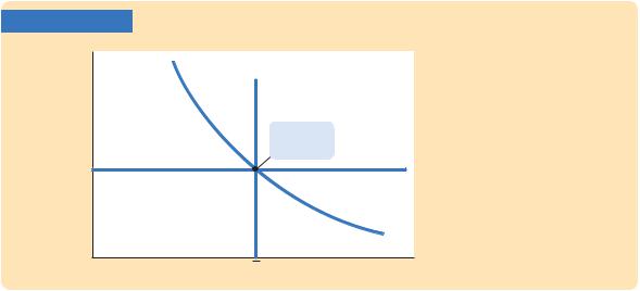
How does the economy make the transition from the short run to the long run? Let’s trace the effects over time of a fall in aggregate demand. Suppose that the economy is initially in long-run equilibrium, as shown in Figure 9-11. In this
FIGURE 9-11
Price level, P
LRAS
Long-run equilibrium
Long-Run Equilibrium In the long run, the economy finds itself at the intersection of the long-run aggregate supply curve and the aggregate demand curve. Because prices have adjusted to this level, the
SRAS short-run aggregate supply curve crosses this point as well.
AD
YIncome, output, Y
276 | P A R T I V Business Cycle Theory: The Economy in the Short Run
figure, there are three curves: the aggregate demand curve, the long-run aggregate supply curve, and the short-run aggregate supply curve. The long-run equilibrium is the point at which aggregate demand crosses the long-run aggregate supply curve. Prices have adjusted to reach this equilibrium. Therefore, when the economy is in its long-run equilibrium, the short-run aggregate supply curve must cross this point as well.
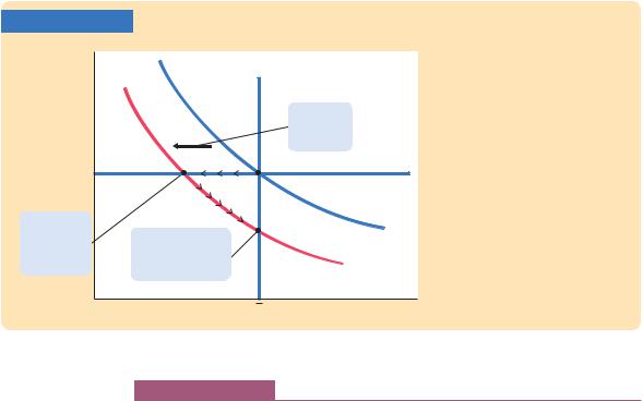
Now suppose that the Fed reduces the money supply and the aggregate demand curve shifts downward, as in Figure 9-12. In the short run, prices are sticky, so the economy moves from point A to point B. Output and employment fall below their natural levels, which means the economy is in a recession. Over time, in response to the low demand, wages and prices fall. The gradual reduction in the price level moves the economy downward along the aggregate demand curve to point C, which is the new long-run equilibrium. In the new long-run equilibrium (point C), output and employment are back to their natural levels, but prices are lower than in the old long-run equilibrium (point A). Thus, a shift in aggregate demand affects output in the short run, but this effect dissipates over time as firms adjust their prices.
FIGURE 9-12
Price level, P
2. ... lowers output in the short run ...
LRAS |
|
|
1. A fall in |
|
aggregate |
|
demand ... |
A |
SRAS |
B |
|
C |
AD1 |
3. ... but in the |
|
long run affects |
AD2 |
only the price level. |
A Reduction in Aggregate Demand The economy begins in long-run equilibrium at point A. A reduction in aggregate demand, perhaps caused by a decrease in the money supply, moves the economy from point A to point B, where output is below its natural level. As prices fall, the economy gradually recovers from the recession, moving from point B to point C.
YIncome, output, Y
CASE STUDY
A Monetary Lesson from French History
Finding modern examples to illustrate the lessons from Figure 9-12 is hard. Modern central banks are too smart to engineer a substantial reduction in the money supply for no good reason. They know that a recession would ensue,

C H A P T E R 9 Introduction to Economic Fluctuations | 277
and they usually do their best to prevent that from happening. Fortunately, history often fills in the gap when recent experience fails to produce the right experiment.
A vivid example of the effects of monetary contraction occurred in eighteenth-century France. François Velde, an economist at the Federal Reserve Bank of Chicago, recently studied this episode in French economic history.
The story begins with the unusual nature of French money at the time. The money stock in this economy included a variety of gold and silver coins that, in contrast to modern money, did not indicate a specific monetary value. Instead, the monetary value of each coin was set by government decree, and the government could easily change the monetary value and thus the money supply. Sometimes this would occur literally overnight. It is almost as if, while you were sleeping, every $1 bill in your wallet was replaced by a bill worth only 80 cents.
Indeed, that is what happened on September 22, 1724. Every person in France woke up with 20 percent less money than they had the night before. Over the course of seven months of that year, the nominal value of the money stock was reduced by about 45 percent. The goal of these changes was to reduce prices in the economy to what the government considered an appropriate level.
What happened as a result of this policy? Velde reports the following consequences:
Although prices and wages did fall, they did not do so by the full 45 percent; moreover, it took them months, if not years, to fall that far. Real wages in fact rose, at least initially. Interest rates rose. The only market that adjusted instantaneously and fully was the foreign exchange market. Even markets that were as close to fully competitive as one can imagine, such as grain markets, failed to react initially. . . .
At the same time, the industrial sector of the economy (or at any rate the textile industry) went into a severe contraction, by about 30 percent. The onset of the recession may have occurred before the deflationary policy began, but it was widely believed at the time that the severity of the contraction was due to monetary policy, in particular to a resulting “credit crunch” as holders of money stopped providing credit to trade in anticipation of further price declines (the “scarcity of money” frequently blamed by observers). Likewise, it was widely believed (on the basis of past experience) that a policy of inflation would halt the recession, and coincidentally or not, the economy rebounded once the nominal money supply was increased by 20 percent in May 1726.
This description of events from French history fits well with the lessons from modern macroeconomic theory.4 ■
4 François R. Velde, “Chronicles of a Deflation Unforetold,” Federal Reserve Bank of Chicago, November 2006.