

C H A P T E R 7 Economic Growth I: Capital Accumulation and Population Growth | 197
FIGURE 7-4
Investment and |
|
Depreciation, dk |
depreciation |
|
|
|
|
|
dk2 |
|
|
i2 |
|
Investment, |
i* dk* |
|
sf(k) |
i1 |
|
|
dk1 |
|
|
|
|
|
|
|
|
k1  k*
k*  k2 Capital
per worker, k
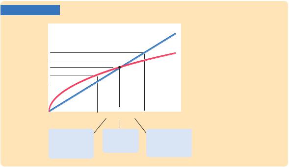
Investment, Depreciation, and the Steady State The steady-state level of capital k* is the level at which investment equals depreciation, indicating that the amount of capital will not change over time. Below k* investment exceeds depreciation, so the capital stock grows. Above k* investment is less than depreciation, so the capital stock shrinks.
Capital stock |
Steady-state |
Capital stock |
increases because |
level of capital |
decreases because |
investment exceeds |
per worker |
depreciation |
depreciation. |
|
exceeds investment. |
an economy not at the steady state will go there. That is, regardless of the level of capital with which the economy begins, it ends up with the steady-state level of capital. In this sense, the steady state represents the long-run equilibrium of the economy.
To see why an economy always ends up at the steady state, suppose that the economy starts with less than the steady-state level of capital, such as level k1 in Figure 7-4. In this case, the level of investment exceeds the amount of depreciation. Over time, the capital stock will rise and will continue to rise—along with output f(k)—until it approaches the steady state k*.
Similarly, suppose that the economy starts with more than the steady-state level of capital, such as level k2. In this case, investment is less than depreciation: capital is wearing out faster than it is being replaced. The capital stock will fall, again approaching the steady-state level. Once the capital stock reaches the steady state, investment equals depreciation, and there is no pressure for the capital stock to either increase or decrease.
Approaching the Steady State: A Numerical Example
Let’s use a numerical example to see how the Solow model works and how the economy approaches the steady state. For this example, we assume that the production function is
Y = K 1/2L1/2.
From Chapter 3, you will recognize this as the Cobb–Douglas production function with the capital-share parameter a equal to 1/2. To derive the per-worker
198 | P A R T I I I Growth Theory: The Economy in the Very Long Run
production function f(k), divide both sides of the production function by the labor force L:
Y |
|
K1/2L1/2 |
|
|
= . |
||
L |
|
L |
|
Rearrange to obtain |
|
|
|
Y |
|
K |
1/2 |
L |
= ( L ) |
. |
|
Because y = Y/L and k = K/L, this equation becomes
y = k1/2,
which can also be written as
y = k.
This form of the production function states that output per worker equals the square root of the amount of capital per worker.
To complete the example, let’s assume that 30 percent of output is saved (s = 0.3), that 10 percent of the capital stock depreciates every year (d = 0.1), and that the economy starts off with 4 units of capital per worker (k = 4). Given these numbers, we can now examine what happens to this economy over time.
We begin by looking at the production and allocation of output in the first year, when the economy has 4 units of capital per worker. Here are the steps we follow.
■According to the production function y = k, the 4 units of capital per worker (k) produce 2 units of output per worker (y).
■Because 30 percent of output is saved and invested and 70 percent is consumed, i = 0.6 and c = 1.4.
■Because 10 percent of the capital stock depreciates, dk = 0.4.
■With investment of 0.6 and depreciation of 0.4, the change in the capital stock is Dk = 0.2.
Thus, the economy begins its second year with 4.2 units of capital per worker. We can do the same calculations for each subsequent year. Table 7-2 shows how the economy progresses. Every year, because investment exceeds depreciation, new capital is added and output grows. Over many years, the economy approaches a steady state with 9 units of capital per worker. In this steady state, investment of 0.9 exactly offsets depreciation of 0.9, so the capital stock and out-
put are no longer growing.
Following the progress of the economy for many years is one way to find the steady-state capital stock, but there is another way that requires fewer calculations. Recall that
Dk = sf(k) − dk.
This equation shows how k evolves over time. Because the steady state is (by definition) the value of k at which Dk = 0, we know that
0 = sf (k*) − dk*,

C H A P T E R 7 Economic Growth I: Capital Accumulation and Population Growth | 199
TA B L E 7-2
Approaching the Steady State: A Numerical Example
|
Assumptions: |
y = k; s = 0.3; |
d = 0.1; initial k = 4.0 |
|
|
|
||
|
Year |
k |
y |
c |
i |
dk |
Dk |
|
1 |
4.000 |
2.000 |
1.400 |
0.600 |
0.400 |
0.200 |
||
2 |
4.200 |
2.049 |
1.435 |
0.615 |
0.420 |
0.195 |
|
|
3 |
4.395 |
2.096 |
1.467 |
0.629 |
0.440 |
0.189 |
|
|
4 |
4.584 |
2.141 |
1.499 |
0.642 |
0.458 |
0.184 |
|
|
5 |
4.768 |
2.184 |
1.529 |
0.655 |
0.477 |
0.178 |
|
|
. |
|
|
|
|
|
|
|
|
. |
|
|
|
|
|
|
|
|
. |
|
|
|
|
|
|
|
|
10 |
5.602 |
2.367 |
1.657 |
0.710 |
0.560 |
0.150 |
|
|
. |
|
|
|
|
|
|
|
|
. |
|
|
|
|
|
|
|
|
. |
|
|
|
|
|
|
|
|
25 |
7.321 |
2.706 |
1.894 |
0.812 |
0.732 |
0.080 |
||
. |
|
|
|
|
|
|
|
|
. |
|
|
|
|
|
|
|
|
. |
|
|
|
|
|
|
|
|
100 |
8.962 |
2.994 |
2.096 |
0.898 |
0.896 |
0.002 |
||
. |
|
|
|
|
|
|
|
|
. |
|
|
|
|
|
|
|
|
. |
|
|
|
|
|
|
|
|
|
9.000 |
3.000 |
2.100 |
0.900 |
0.900 |
0.000 |
||
|
|
|
|
|
|
|
|
|
or, equivalently,
k* s
= . f(k*) d
This equation provides a way of finding worker, k*. Substituting in the numbers example, we obtain
the steady-state level of capital per and production function from our
k* 0.3
= .
k* 0.1
Now square both sides of this equation to find
k* = 9.
The steady-state capital stock is 9 units per worker. This result confirms the calculation of the steady state in Table 7-2.

200 | P A R T I I I Growth Theory: The Economy in the Very Long Run
CASE STUDY
The Miracle of Japanese and German Growth
Japan and Germany are two success stories of economic growth. Although today they are economic superpowers, in 1945 the economies of both countries were in shambles. World War II had destroyed much of their capital stocks. In the decades after the war, however, these two countries experienced some of the most rapid growth rates on record. Between 1948 and 1972, output per person grew at 8.2 percent per year in Japan and 5.7 percent per year in Germany, compared to only 2.2 percent per year in the United States.
Are the postwar experiences of Japan and Germany so surprising from the standpoint of the Solow growth model? Consider an economy in steady state. Now suppose that a war destroys some of the capital stock. (That is, suppose the capital stock drops from k* to k1 in Figure 7-4.) Not surprisingly, the level of output falls immediately. But if the saving rate—the fraction of output devoted to saving and investment—is unchanged, the economy will then experience a period of high growth. Output grows because, at the lower capital stock, more capital is added by investment than is removed by depreciation. This high growth continues until the economy approaches its former steady state. Hence, although destroying part of the capital stock immediately reduces output, it is followed by higher-than-normal growth. The “miracle’’ of rapid growth in Japan and Germany, as it is often described in the business press, is what the Solow model predicts for countries in which war has greatly reduced the capital stock. ■
How Saving Affects Growth
The explanation of Japanese and German growth after World War II is not quite as simple as suggested in the preceding case study. Another relevant fact is that both Japan and Germany save and invest a higher fraction of their output than does the United States. To understand more fully the international differences in economic performance, we must consider the effects of different saving rates.
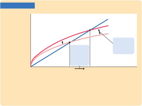
Consider what happens to an economy when its saving rate increases. Figure 7-5 shows such a change. The economy is assumed to begin in a steady state with saving rate s1 and capital stock k*1. When the saving rate increases from s1 to s2, the sf(k) curve shifts upward. At the initial saving rate s1 and the initial capital stock k*1, the amount of investment just offsets the amount of depreciation. Immediately after the saving rate rises, investment is higher, but the capital stock and depreciation are unchanged. Therefore, investment exceeds depreciation. The capital stock will gradually rise until the economy reaches the new steady state k*2, which has a higher capital stock and a higher level of output than the old steady state.
The Solow model shows that the saving rate is a key determinant of the steady-state capital stock. If the saving rate is high, the economy will have a large capital stock and a high level of output in the steady state. If the saving rate is low, the econ-
C H A P T E R 7 Economic Growth I: Capital Accumulation and Population Growth | 201
FIGURE 7-5
Investment
and depreciation
|
dk |
|
s2f(k) |
|
s1f(k) |
|
1. An increase |
|
in the saving |
2. ... causing |
rate raises |
the capital |
investment, ... |
stock to grow |
|
toward a new |
|
steady state. |
|
k* |
k* |
Capital |
1 |
2 |
per worker, k |
|
|
An Increase in the Saving Rate An increase in the saving rate s implies that the amount of investment for any given capital stock is higher. It therefore shifts the saving function upward. At the initial
steady state k*, investment now exceeds depreciation. The capital
1
stock rises until the economy reaches a new steady state k* with more
2
capital and output.
omy will have a small capital stock and a low level of output in the steady state. This conclusion sheds light on many discussions of fiscal policy. As we saw in Chapter 3, a government budget deficit can reduce national saving and crowd out investment. Now we can see that the long-run consequences of a reduced saving rate are a lower capital stock and lower national income. This is why many economists are critical of persistent budget deficits.
What does the Solow model say about the relationship between saving and economic growth? Higher saving leads to faster growth in the Solow model, but only temporarily. An increase in the rate of saving raises growth only until the economy reaches the new steady state. If the economy maintains a high saving rate, it will maintain a large capital stock and a high level of output, but it will not maintain a high rate of growth forever. Policies that alter the steady-state growth rate of income per person are said to have a growth effect; we will see examples of such policies in the next chapter. By contrast, a higher saving rate is said to have a level effect, because only the level of income per person—not its growth rate—is influenced by the saving rate in the steady state.
Now that we understand how saving and growth interact, we can more fully explain the impressive economic performance of Germany and Japan after World War II. Not only were their initial capital stocks low because of the war, but their steady-state capital stocks were also high because of their high saving rates. Both of these facts help explain the rapid growth of these two countries in the 1950s and 1960s.
202 | P A R T I I I Growth Theory: The Economy in the Very Long Run
CASE STUDY
Saving and Investment Around the World
We started this chapter with an important question: Why are some countries so rich while others are mired in poverty? Our analysis has taken us a step closer to the answer. According to the Solow model, if a nation devotes a large fraction of its income to saving and investment, it will have a high steady-state capital stock and a high level of income. If a nation saves and invests only a small fraction of its income, its steady-state capital and income will be low.
Let’s now look at some data to see if this theoretical result in fact helps explain the large international variation in standards of living. Figure 7-6 is a scatterplot of data from 96 countries. (The figure includes most of the world’s economies. It excludes major oil-producing countries and countries that were communist during much of this period, because their experiences are explained by their spe-
FIGURE 7-6
Income per person in 2003 (logarithmic scale)
100,000
10,000
1,000
100
|
|
|
|
|
|
|
|
|
|
|
|
|
|
|
|
|
|
|
|
Luxembourg |
Switzerland |
|||||||||||||||
|
|
|
|
|
|
|
|
|
|
|
|
|
|
|
|
|
|
|
|
|||||||||||||||||
|
|
|
|
|
|
|
|
|
|
|
United States |
|
|
|||||||||||||||||||||||
|
|
|
|
|
|
|
|
|
|
|
|
|
|
|
|
|
|
|
|
Norway |
||||||||||||||||
|
|
|
|
|
|
|
|
United Kingdom |
|
|
|
|
|
|
|
|
|
|
|
|
|
|
||||||||||||||
|
|
Barbados |
|
|
|
|
|
|
|
|
|
|
|
|
|
|
|
|
|
|
|
|
|
|
|
|
|
|
Japan |
|||||||
|
|
|
Argentina |
|
|
|
|
|
|
|
|
|
|
|
Finland |
|||||||||||||||||||||
|
|
|
|
|
|
|
|
|
|
|
|
|
|
|
|
|
|
|
|
|
Spain |
|
|
|
|
|
|
|
|
|
|
|
|
|
||
|
|
|
|
|
|
|
South Africa |
|
|
|
|
|
|
|
|
|
|
|
|
|
|
|
|
South Korea |
||||||||||||
|
|
|
|
|
|
|
|
|
|
|
|
|
|
|
|
|
|
|
|
|
|
|
|
Greece |
||||||||||||
|
|
|
|
|
|
|
|
|
|
|
|
|
|
|
|
|
Mexico |
|
|
|
|
|
|
Thailand |
||||||||||||
|
|
El Salvador |
|
|
|
|
|
|
|
|
|
|
Peru |
|
|
|
|
|
China |
|||||||||||||||||
|
Cameroon |
|
|
|
|
|
|
|
|
|
|
|
|
|
|
|
|
|
|
|
|
|
|
|
|
|
|
|
|
|
|
|
|
|
||
|
|
|
|
|
|
|
Pakistan |
|
|
|
|
Ecuador |
||||||||||||||||||||||||
Rwanda |
|
|
|
|
|
|
|
|
|
|
|
|
|
|
|
|
|
|
|
|
|
|
|
|
|
|
|
|||||||||
|
|
|
|
India |
|
|
|
|
|
|
|
|
|
|
|
|
|
|
|
|
|
|
|
|
|
|
|
|
|
|
|
|
|
|||
|
|
|
|
|
|
Nigeria |
|
Ghana |
|
|
|
|
|
|
|
Republic of Congo |
||||||||||||||||||||
|
|
|
|
|
|
|
|
|
|
|
|
|
|
|
|
|
|
|
|
|
|
|
|
|
|
|
|
|
|
|
|
|
|
|
Zambia |
|
|
|
|
|
|
|
|
Togo |
|
|
|
|
|
|
|
|
|
|
|
|
|
|
|
|
|
|
|
|
|
|
|
|
|
|
|
|
|
|
|
|
|
|
Burundi |
|
Guinea-Bissau |
|
|
|
|
|
|
|
|
|
|
|
|
|
|
|
|
|
|
|
|
|||||||||
|
Ethiopia |
|
|
|
|
|
|
|
|
|
|
|
|
|
|
|
|
|
|
|
|
|
|
|
|
|
|
|
|
|
|
|
|
|
||
|
|
|
|
|
|
|
|
|
|
|
|
|
|
|
|
|
|
|
|
|
|
|
|
|
|
|
|
|
|
|
|
|
|
|
|
|
|
|
|
|
|
|
|
|
|
|
|
|
|
|
|
|
|
|
|
|
|
|
|
|
|
|
|
|
|
|
|
|
|
|
|
|
|
0 |
5 |
10 |
15 |
20 |
25 |
30 |
35 |
Investment as percentage of output (average 1960–2003)
International Evidence on Investment Rates and Income per Person This scatterplot shows the experience of 96 countries, each represented by a single point. The horizontal axis shows the country’s rate of investment, and the vertical axis shows the country’s income per person. High investment is associated with high income per person, as the Solow model predicts.
Source: Alan Heston, Robert Summers, and Bettina Aten, Penn World Table Version 6.2, Center for International Comparisons of Production, Income and Prices at the University of Pennsylvania, September 2006.